Download
1 / 37
380 likes | 506 Views
This overview covers the essential principles of customer research and market segmentation, emphasizing how heterogeneous markets can be effectively segmented. Key definitions, conditions for creating segmentation opportunities, requirements for effective segmentation, and a detailed five-step segmentation process are discussed. Furthermore, the paper explores proactive versus reactive segmentation strategies, along with essential techniques such as factor analysis. Insight into various statistics associated with factor analysis, including correlation matrices and factor loadings, is provided to enhance understanding.

E N D
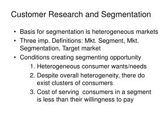
Customer Research and Segmentation • Basis for segmentation is heterogeneous markets • Three imp. Definitions: Mkt. Segment, Mkt. Segmentation, Target market • Conditions creating segmenting opportunity 1. Heterogeneous consumer wants/needs 2. Despite overall heterogeneity, there do exist clusters of consumers 3. Cost of serving consumers in a segment is less than their willingness to pay
Customer Res. & Segmentation • Requirements. For effective segmentation 1. Measurability 2. Accessibility 3. Sustainability 4. Actionability • Segmentation model requires segmentation basis and segment descriptors
Customer Res. & Segmentation • Approach to segmentation depends on problem • Segmentation best described as first step in a 5 step process 1. Segment mkt. using demand variables 2. Describe segments using descriptors 3. Evaluate attractiveness of each segment 4. Select one or more segments to serve 5. Identify positioning concept. • Let us study step 1 in detail
Customer Res. & Segmentation • Segmentation can be reactive or proactive • 5 steps in proactive segmentation 1. Explicitly outline role of segmentation 2. Select segmentation variable 3. Choose statistical procedures 4. Determine max. number of segments 5. Search across segments to see how many of those to target
Factor Analysis © 2007 Prentice Hall
Chapter Outline 1) Overview 2) Basic Concept 3) Factor Analysis Model 4) Statistics Associated with Factor Analysis
Chapter Outline 5) Conducting Factor Analysis • Problem Formulation • Construction of the Correlation Matrix • Method of Factor Analysis • Number of of Factors • Rotation of Factors • Interpretation of Factors • Factor Scores • Model Fit
Factor Analysis • Factor analysis is a class of procedures used for data reduction and summarization. • It is an interdependence technique: no distinction between dependent and independent variables. • Factor analysis is used: • To identify underlying dimensions, or factors, that explain the correlations among a set of variables. • To identify a new, smaller, set of uncorrelated variables to replace the original set of correlated variables.
Factor 2 Baseball Football Evening at home Factor 1 Go to a party Home is best place Plays Movies Factors Underlying Selected Psychographics and Lifestyles Fig. 19.1
Factor Analysis Model Each variable is expressed as a linear combination of factors. The factors are some common factors plus a unique factor. The factor model is represented as: Xi = Ai 1F1 + Ai 2F2 + Ai 3F3 + . . . + AimFm + ViUi where Xi = i th standardized variable Aij = standardized mult reg coeff of var i on common factor j Fj = common factor j Vi = standardized reg coeff of var i on unique factor i Ui = the unique factor for variable i m = number of common factors
Factor Analysis Model • The first set of weights (factor score coefficients) are chosen so that the first factor explains the largest portion of the total variance. • Then a second set of weights can be selected, so that the second factor explains most of the residual variance, subject to being uncorrelated with the first factor. • This same principle applies for selecting additional weights for the additional factors.
Factor Analysis Model The common factors themselves can be expressed as linear combinations of the observed variables. Fi = Wi1X1 + Wi2X2 + Wi3X3 + . . . + WikXk Where: Fi = estimate of i th factor Wi= weight or factor score coefficient k = number of variables
Statistics Associated with Factor Analysis • Bartlett's test of sphericity. Bartlett's test of sphericity is used to test the hypothesis that the variables are uncorrelated in the population (i.e., the population corr matrix is an identity matrix) • Correlation matrix. A correlation matrix is a lower triangle matrix showing the simple correlations, r, between all possible pairs of variables included in the analysis. The diagonal elements are all 1.
Statistics Associated with Factor Analysis • Communality. Amount of variance a variable shares with all the other variables. This is the proportion of variance explained by the common factors. • Eigenvalue. Represents the total variance explained by each factor. • Factor loadings. Correlations between the variables and the factors. • Factor matrix. A factor matrix contains the factor loadings of all the variables on all the factors
Statistics Associated with Factor Analysis • Factor scores. Factor scores are composite scores estimated for each respondent on the derived factors. • Kaiser-Meyer-Olkin (KMO) measure of sampling adequacy. Used to examine the appropriateness of factor analysis. High values (between 0.5 and 1.0) indicate appropriateness. Values below 0.5 imply not. • Percentage of variance. The percentage of the total variance attributed to each factor. • Scree plot. A scree plot is a plot of the Eigenvalues against the number of factors in order of extraction.
Example: Factor Analysis • HATCO is a large industrial supplier • A marketing research firm surveyed 100 HATCO customers, to investigate the customers’ perceptions of HATCO • The marketing research firm obtained data on 7 different variables from HATCO’s customers • Before doing further analysis, the mkt res firm ran a Factor Analysis to see if the data could be reduced
Example: Factor Analysis • In a B2B situation, HATCO wanted to know the perceptions that its customers had about it • The mktg res firm gathered data on 7 variables 1. Delivery speed 2. Price level 3. Price flexibility 4. Manufacturer’s image 5. Overall service 6. Salesforce image 7. Product quality • Each var was measured on a 10 cm graphic rating scale Poor Excellent
Construction of the Correlation Matrix Method of Factor Analysis Determination of Number of Factors Rotation of Factors Conducting Factor Analysis Fig. 19.2 Problem formulation Interpretation of Factors Calculation of Factor Scores Determination of Model Fit
Formulate the Problem • The objectives of factor analysis should be identified. • The variables to be included in the factor analysis should be specified. The variables should be measured on an interval or ratio scale. • An appropriate sample size should be used. As a rough guideline, there should be at least four or five times as many observations (sample size) as there are variables.
Construct the Correlation Matrix • The analytical process is based on a matrix of correlations between the variables. • If the Bartlett's test of sphericity is not rejected, then factor analysis is not appropriate. • If the Kaiser-Meyer-Olkin (KMO) measure of sampling adequacy is small, then the correlations between pairs of variables cannot be explained by other variables and factor analysis may not be appropriate.
Determine the Method of Factor Analysis • In Principal components analysis, the total variance in the data is considered. -Used to determine the min number of factors that will account for max variance in the data. • InCommon factor analysis, the factors are estimated based only on the common variance. -Communalities are inserted in the diagonal of the correlation matrix. -Used to identify the underlying dimensions and when the common variance is of interest.
Determine the Number of Factors • A Priori Determination.Use prior knowledge. • Determination Based on Eigenvalues.Only factors with Eigenvalues greater than 1.0 are retained. • Determination Based on Scree Plot.A scree plot is a plot of the Eigenvalues against the number of factors in order of extraction. The point at which the scree begins denotes the true number of factors. • Determination Based on Percentage of Variance.
Rotation of Factors • Through rotation the factor matrix is transformed into a simpler one that is easier to interpret. • After rotation each factor should have nonzero, or significant, loadings for only some of the variables. Each variable should have nonzero or significant loadings with only a few factors, if possible with only one. • The rotation is called orthogonal rotation if the axes are maintained at right angles.
Rotation of Factors • Varimax procedure. Axes maintained at right angles -Most common method for rotation. -An orthogonal method of rotation that minimizes the number of variables with high loadings on a factor. -Orthogonal rotation results in uncorrelated factors. • Oblique rotation. Axes not maintained at right angles -Factors are correlated. -Oblique rotation should be used when factors in the population are likely to be strongly correlated.
Interpret Factors • A factor can be interpreted in terms of the variables that load high on it. • Another useful aid in interpretation is to plot the variables, using the factor loadings as coordinates. Variables at the end of an axis are those that have high loadings on only that factor, and hence describe the factor.
Calculate Factor Scores The factor scores for the i th factor may be estimated as follows: Fi = Wi1 X1 + Wi2 X2 + Wi3 X3 + . . . + Wik Xk
Determine the Model Fit • The correlations between the variables can be deduced from the estimated correlations between the variables and the factors. • The differences between the observed correlations (in the input correlation matrix) and the reproduced correlations (estimated from the factor matrix) can be examined to determine model fit. These differences are called residuals.
Another Example of Factor Analysis • To determine benefits from toothpaste • Responses were obtained on 6 variables: V1: It is imp to buy toothpaste to prevent cavities V2: I like a toothpaste that gives shiny teeth V3: A toothpaste should strengthen your gums V4: I prefer a toothpaste that freshens breath V5: Prevention of tooth decay is not imp V6: The most imp consideration is attractive teeth • Responses on a 7-pt scale (1=strongly disagree; 7=strongly agree)
Another Example of Factor Analysis Table 19.1
Table 19.2 Correlation Matrix
Results of Principal Components Analysis Table 19.3
Results of Principal Components Analysis Table 19.3, cont.
Results of Principal Components Analysis Table 19.3, cont.
Results of Principal Components Analysis Table 19.3, cont. -The lower-left triangle is correlation matrix; -The diagonal has the communalities; -The upper-right triangle has the residuals between the observed correlations and the reproduced correlations.
3.0 2.5 2.0 Eigenvalue 1.5 1.0 0.5 0.0 1 2 3 4 5 6 Component Number Scree Plot Fig. 19.3
Fig. 19.4 Factors Factors Variables 1 2 3 4 5 6 1 X X X 2 X X X Variables 1 2 3 4 5 6 1 X X X X X 2 X X X X (a) (b) High Loadings Before Rotation High Loadings After Rotation Factor Matrix Before and After Rotation
Factor Loading Plot Fig. 19.5 Rotated Component Matrix Component 1 2 V1 0.962 -2.66E-02 V2 -5.72E-02 0.848 V3 0.934 -0.146 V4 -9.83E-02 0.854 V5 -0.933 -8.40E-02 V6 8.337E-02 0.885 Component Plot in Rotated Space V4 V6 1.0 0.5 0.0 -0.5 -1.0 V2 V1 Component 2 V5 V3 -1.0 -0.5 0.0 0.5 1.0 Component 1