Download
1 / 27
1.48k likes | 6.44k Views
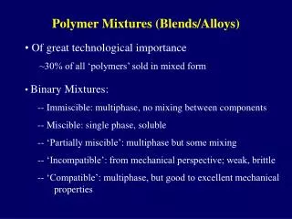
Polymer Mixtures (Blends/Alloys). Of great technological importance ~30% of all ‘polymers’ sold in mixed form Binary Mixtures: -- Immiscible: multiphase, no mixing between components -- Miscible: single phase, soluble -- ‘Partially miscible’: multiphase but some mixing

E N D
Polymer Mixtures (Blends/Alloys) • Of great technological importance ~30% of all ‘polymers’ sold in mixed form • Binary Mixtures: -- Immiscible: multiphase, no mixing between components • -- Miscible: single phase, soluble • -- ‘Partially miscible’: multiphase but some mixing • -- ‘Incompatible’: from mechanical perspective; weak, brittle • -- ‘Compatible’: multiphase, but good to excellent mechanical properties
What’s So Special About Polymer Blends? • Multiphase • Economics • Enhanced mechanical properties • eg. PS/PB (5-20%) • -- Mechanical blend: no increase in impact properties (‘incompatible’) • -- PB dispersed in styrene then polymerize PS, PB, • PS-g-PB (‘compatiblizer’ (surfactant) , few %) [HIPS] • - ‘phase within a phase within a phase’ morphology • mechanically toughen • -- ABS similar
Why Should We Care About Blends? (con’d) ‘Added’ graft or block Notched Izod PS 0.25 – 0.4 (ft-lb/in) HIPS 0.5 – 4 but E and b as rubber Impact strength Blend Elastomer % ~5 - 15% • Why enhancement of impact strength? • rubber particles act as stress concentrators to initiate matrix yielding (crazing &/or shear yielding)
Mechanism of Rubber Toughening in Thermoplastic Polymers • Mechanism of energy absorption: initially brittle polymers (e.g. PS, PMMA) • a. Rubber particles act to initiate very large number (~106) of crazes in glassy matrix • b. Crazes grow until they encounter another rubber particle or craze • Energy consumed principally in plastic deformation of matrix • c. Rubber particles act as craze termination points and obstacles to craze or crack propagation
HIPS TEM OsO4 staining for contrast Dark = PB PS inclusions in ‘rubber’ particles Wagner and Robeson (1970)
direction HIPS (con’d) • Crazing in thin HIPS film Rubber particle: PS inclusions What are crazes?
direction ABS: Acrylonitrile - Styrene - Butadiene TEM Synthesis? Dispersed phase particle size ~0.1 - 0.5 m
Rubber Toughening (con’d) • Important features required to produce good impact properties: • a. elastomer must phase separate and be dispersed randomly as small discrete particles • b. elastomer must have low Tg (Tg << Ttest) • c. good interfacial adhesion ('compatibilizers') • d. low shear modulus in relation to matrix • What toughening mechanism often operates to toughen ‘quasi-ductile’ polymers (e.g. that lead to ‘super tough’ nylons or polyacetals)?
Why Should We Care AboutMiscible Blends? • Miscible mixtures: • - No interfaces to contend with • - Cost/property combination (e.g. Noryl [PPO/PS]) • - Macromolecular plasticizer or other additive (non-migrating) • - In some cases, modest ‘synergism’ in some mechanical properties • - Model systems for fundamental studies
Phase Diagrams Phase Behavior f (T, P, Vi) Upper Critical Soln Temp. (UCST) - binodal (coexistence curve) boundary between stable & unstable - spinodal: boundary between metastable & unstable Critical point -- Quench into 2 phase region compositions along binodal define composition of phases (lever rule)
Phase Diagrams (con’d) • Lower Critical Soln Temp. (LCST) • -- Binodal • -- Spinodal • Difference between metastable & unstable regions? • -- mechanism of phase decomposition (spinodal decomposition vs. nucleation and growth)
Phase Diagrams (con’d) ‘Hourglass’- merging of LCST & UCST Both LCST & UCST Closed loop behavior
Gmix (= Hmix – T Smix) as f(T,P,V1) • Theory of polymer solutions: • Flory-Huggins (polymer + solvent) lattice model; emphasis on calculation of Sm • Extension to polymer-polymer mixtures [Scott, (1949)] • Improved theories (e.g. eqn of state theories [Flory (1970)]; inclusion of strong intermolecular interactions: lattice fluid; group contributions, etc) Understanding Miscibility andPhase Behavior
Simplified Theory of Polymer Solutions* 1. Polymer/solvent UCST & LCST 2. Polymer/polymer a) dispersive forces (Hm > 0) single phase only if MW < few 1000 (UCST) b) strong interactions (Hm < 0) miscible at high MW (LCST) 3. Two miscible polymers + solvent (possible to get phase separation in ternary mix even if all 3 binaries are miscible, if large difference in affinities of polymers for solvent (“effect”) 4. Two strongly interacting polymers (miscible) + solvent (possible to get phase separation in ternary mixture if polymer - polymer interactions become very large) *Patterson & Robard, Macromolecules (1978); Patterson, PES (1982)
Sm (S-S) > Sm (S-P) > Sm (P-P) Important Contributions to Gmix • Combinatorial Smix;intermolecular interactions (contact energy); ‘free volume’ effects • 1. Combinatorial Smix Sm related to # of permutations of molecules of liquid among sites on soln) ‘quasi-lattice’, i.e., positional disorder Sm =k ln always + entropic stabilization
Regular Solution Theory for Small Molecules -Sm/R = N1 lnX1 + N2 lnX2 Not appropriate for polymers: Equivalent to assuming solvent & entire polymer occupy 1 lattice site Rather, define: Vsolv = Ns Vs / (Ns Vs + MNpVs) Polymer defined = chain of segments which have same vol as solvent M = vol. occupied by poly vol. occupied by solvent M = not necessarily = DP Mole fraction Vol. fraction (s) # segments in poly # molecules or moles
Entropic stabilization: P - P 0, in the limit of MW for both Entropic stabilization: P - S (V2 0) Soln more stable at high [P]?? Entropic stabilization: S - S composition Flory – Huggins Sm/R = -[N1 lnV1 + N2 lnV2] Mix N1 moles of #1 with N2 moles #2: On per volume of soln basis (V): Assume V1 = V2 = 1/2, & for solvent/solvent V1 ~ V2 ~ 100 cc/mol: Molar volumes
+ Gm 0 > Free Energy and Phase Separation Mixture can develop lower Gm by separating into 2 phases V2 At a given T and P • Phase separation occurs if Gm becomes concave downward i.e., if • Thermodynamic criteria for miscibility: • Gmand
Related to weakness or strength of 1-2 contacts relative to 1-1 & 2-2 • Flory: • Hm/RTV = (z W12 kTVs) V1V2 = (12 V1) V1V2 • characterizes the interaction energy lattice coordination number Exchange energy for breaking 1/1& 2/2 contacts & forming 1/2 2. Interactional Contribution = 1/2(W11 +W22) -W12 Vs = molar vol of segment (of S in P/S) Interaction parameter # segments in 1 (= S in P/S) Dispersive 1-2 contacts + Hm Strong Interactions - Hm important in poly/poly mixing
combinatorialinteractional for polymer/polymer (r1 ) 12 ! Important quality 12 / r1 or12 / V1 independent of MW Total Free Energy of Mixing Gm/RTV = [V1 lnV1 V1 + V2 lnV2 V2] +(12 V1) V1V2 Another common form: Gm/RT = [V1 lnV1 M1 + V2 lnV2 M2] + 12 V1V2 “DP” Defined as per segment - normally used in the literature Gm per mole of lattice sites
Typical Polymer Solution (in LMW solvent) (12 V1) V1V2 for 12 > 0 Total Gm for polymer/solvent Total Gm for polymer/polymer with dispersive forces Concave downward throughout entire composition range (phase separate into pure 1&2)
12 V1 + 0 Temperature Dependence of 12 12 ~ T-1 For dispersive forces 12 r1 = z W12 kT For strong interactions For a given composition Temperature
Arises as a consequence of –Vmix & related to difference in coefficient of thermal expansion of components • Negative contribution to Hm and Smpositive contribution to Gm (destabilizing) • It’s the non-combinational Sm that derives phase separation at high T in polymer-polymer (LCST has hence been termed an entropy driven process) • Free volume effects get collected in 12 along with interactions • As T , Vfree difference between solvent & polymer (or 2 polymers) increases, as does the positive contribution to 12 3. Free Volume Contribution Vmix 0 Soln has free vol closer to polymer
If 12 independent of concentration: • (12 V1)crit = 1/2 [V1-0.5 + V2-0.5]2 • Both low MW; from regular soln theory of small molecule mixs: Critical Points Also equivalent expression where molar volumes replaced with M’s i.e., 12> 2 phase separated
Polymer/solvent • V2 (i.e., MW ) (12 V1)crit • Polymer/polymer V1 &V2 0; (12 V1)crit 0 3. Critical Points (con’d)
Phase Behavior critdecreases as MW increases 0 c = a + b (dispersive forces) LCST and UCST d = a + b (strong interactions dominate) For given composition
Interplay of combinational Sm, interactions, and Vfree contributions, as function of T and composition, determine whether system will be single or multiphase + allows qualitative description of phase behavior of polymer mixtures (P-S and P-P) For high MW P-P mixtures, simple theory suggests that strong interactions required to obtain single phase state at given T (and these mixtures will phase separate on increasing T) Initial Summary