Two Main Uses of Statistics:

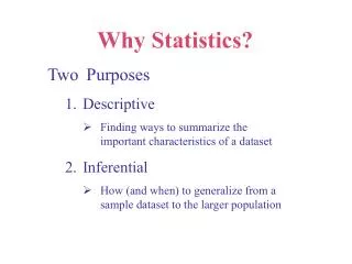
1. Two Main Uses of Statistics: Descriptive: To describe or summarize a collection of data points The data set in hand = the population of interest Inferential: To make decisions or draw conclusions under conditions of uncertainty and incompleteness The data set in hand = a sample or an indicator of some larger population of interest Use these data to make an “educated guess” (or calculated guess) about what we would find if we had full information Use the mathematical idea of probability to make calculated guesses with plausible degrees of certainty

2. Probability (the key concept): Probability = mathematical construct: An idealized theory about hypothetical data Use probability theory to develop mathematical models of these data Many physical events display patterns that follow these mathematical models Apply approximately & “in the long run” Use these models to make predictions & decisions about real world outcomes (with a calculated chance of error or uncertainty) This represents “rational decision-making” – i.e., making uncertain but calculated guesses

3. Probability (cont.): Definition: Probability of an outcome = # of occurrences of specific outcome . # of all possible outcomes E.g., flipping a coin and getting “heads” (1/2) A mathematical expectation of what happens “in the (infinitely) long run” Note difference between probabilities and frequencies Probabilities= calculated and idealized (expected) Frequencies = measured and counted (observed) Arithmetic of probabilities Can be combined (by adding or multiplying) Probabilities of all possible outcomes sum to 1.0 Used to predict likelihood of complex events

5. Probability Distribution: Refers to the distribution of all possible outcomes by the likelihood of each one occurring (similar to frequency distribution) Sum of all these likelihoods = 1.0 Note difference between: Discrete outcomes A specific number of values each with a specific probability The specific probabilities add up to 1.0 Continuous outcomes An infinite number of possible values each with a near-zero probability (of being exactly that value) Described by a probability density function where “probability density” = mathematical likelihood of being in that area

6. Probabilities of a Discrete Variable

7. Probability Density Probability Density function for a Continuous Variable

8. Probability Distributions: We can describe probability distributions the same way as we describe frequency distributions – e.g., central tendency, dispersion, symmetry – depending on the type of variable Characteristics of probability distributions are called parameters and they are referenced by Greek letters (as mathematical idealizations) – e,g, σ2 These compare to measured characteristics of frequency distributions (which are referenced by ordinary English letters) – s2

9. Probability Distributions: Many different probability distributions are possible, each with its own unique likelihood function and its own generating function A few have proven very useful because: They seem to fit well to observed and naturally occurring patterns They are calculable and usable Most famous & useful = Normal Distribution Shows up in many naturally occurring patterns Constitute the “limiting form” of many different distributions (as their numbers get larger) Probabilities can be exactly calculated

10. The Normal Distribution: A very specific probability distribution with its own unique likelihood function that: Yields a completely symmetric distribution that always has the same “bell” shape” curve (relating values to probabilities) (i.e., the Normal Curve) Contains only 2 parameters which exactly determine the size of every Normal distribution: μ (central tendency) (Greek letter mu) (= the mean) σ (dispersion around the center) (Greek letter sigma) (= the standard deviation)

11. 3 different normal distributions

12. The Normal Distribution: Very well known with exactly calculated probabilities (prob. Densities) +1σ 68% +2σ 95% +3σ 99.7% All normal distributions fit exactly this probability curve We can use the normal curve to determine how unusual or unlikely different scores are But to be useful, they need to be converted to a common standard metric (or units)

13. The Normal Distribution: We need to know the parameters of population’s distribution of scores:μ &σ With these, we can covert the scores to a standard normal distribution Where scores = deviations from the mean :μ And expressed in σ units Convert scores into standard scores by: Z = X – μ (“Z Scores”) σ Look up compute Z-score in Normal Table (e.g., Appendix C – Table A)

14. The Normal Distribution (cont): Score from Normal Distribution Table tells proportion of scores above and below the specific (standardized) data value. E.g., a score of 125 on IQ test where μ = 100 & σ = 10  Z = +2.5 What % of scores are below this score? What % are above it? E.g., a score of 75 on IQ test where μ = 100 & σ = 10  Z = -2.5 What % of scores are below this score? What % are above it?