Download
1 / 31
370 likes | 634 Views
Introduction of the F=1 spinor BEC. 郭西川 國立彰化師範大學物理系. Spinor BEC. hyperfine spin. electron spin. nuclear spin. magnetic trapping (one-component, scalar). BEC. optical trapping (multi-component, vector). F=1 spinor BEC : 23 Na, 87 Rb,.

E N D
Introduction of the F=1 spinor BEC 郭西川 國立彰化師範大學物理系
Spinor BEC hyperfine spin electron spin nuclear spin magnetic trapping (one-component, scalar) BEC optical trapping (multi-component, vector) F=1 spinor BEC :23Na, 87Rb,...
Grand canonical energy-functional for the spinor BEC (Ho, Ohmi) N is a fixed number (gs<0: ferromagnetic; gs>0: antiferromagnetic)
order parameter: global phase rotational symmetry in spin space spin operators:
Ground state structure of spinor BEC Define the normalized spinor by Such that all spinors are degenerate with the transformation where Euler angles
Define then the free energy can be expressed as The free energy of K is minimized by:
Coupled GPE for spinor BEC Time-dependent coupled GPE
Modification of GPE – conservation of magnetization The spin-exchange interaction also preserves the magnetization M, so we have two constraints for the GPE
The conservation of particle number and magnetization is equivalent to introduce the Lagrange multipliers and B in the free energy N and M areboth fixed numbers
Some interesting results Ferromagnetic: 3 identical decoupled equations anti-ferromagnetic: 2 coupled-mode equations
Field-induced phase segregation of the condensate configuration the spin configuration of Using the inequality the ground state can be constructed by minimizing the spin-dependent part of the Hamiltonian Case 1: Choose However, since (ferromagnetic state)
Let (Larmor frequency) the Hamiltonian is invariant under the gauge transformation
Case 2: so that we have Choose The minimum is achieved if We may assume that 0 and is real but since which is in contraction with the condition and we must conclude that
For (polar state ) where the condition Note that when cannot be fulfilled and we must chooseFsuch that is as close to as possible. This implies that and thus the ground state is described by (ferromagnetic state )
For the two different configurations coexist: (polar region) (ferro region) The phase boundary rb is determined by
The free energy is given by In the Thomas-Fermi limit, the minimization of the free energy, leads to
Example: phase boundary radius of atomic cloud The total particle number and the chemical potential is related by
Derivation of hydrodynamic equations collective excitations polar region hydrodynamic-like mode ferro region fluctuation of number density Furthermore, we let fluctuation of spin density
Substituting into the time-dependent GP equation Upon linearization we obtain the hydrodynamic equations in different regions: ferro region (Stringari) polar region
Example: where Now let
To solve the coupled equations, let and we obtain the recursion relation Denote u as the eigenvectors of A with eigenvalues and let
Boundary condition requires that the series must terminate at some interger k=2n and the solution is The dispersion relations do not depend on the magnetic field!
L-independence of solutions of polynomial-type Consider a general quadratic potential where the 33 matrix (ij) is positively definite. Consider a polynomial solution where Pk(r) and Qk(r) are homogeneous polynomials of degree k.
Note that if Pk(r) is a polynomial of x,y,z with degree k is a polynomial of degree k-2 is a polynomial of degree k Clearly, terms of even degree are decoupled from terms of odd degree. So we may assume Collecting terms of degree n on both sides The obtained frequency does not depend on L
In memory of Prof. W.-J. Huang (黃文瑞) —A friend and a tutor
Gross-Pitaeviski Hamlitonian for the spinor BEC(Ho, Ohmi) (gs<0: ferromagnetic; gs>0: antiferromagnetic)