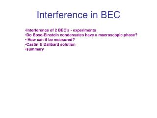
Interference in BEC
Interference in BEC. Interference of 2 BEC’s - experiments Do Bose-Einstein condensates have a macroscopic phase? How can it be measured? Castin & Dalibard solution summary. Separation between the 2 condensates = d. Relative velocity in the x direction ~ d/t. Interference fringes.

Interference in BEC
E N D
Presentation Transcript
Interference in BEC • Interference of 2 BEC’s - experiments • Do Bose-Einstein condensates have a macroscopic phase? • How can it be measured? • Castin & Dalibard solution • summary
Separation between the 2 condensates = d Relative velocity in the x direction ~ d/t
‘giant matter wave’ interference andrews et. el. Science 31 / 1/ 1997 “closing one slit”
GPE calculation Degenerate ground state φ=i2πpx/h+ φ0 z r
A simple model (Castin 2003) Initial state : Ka Kb There is no relative phase between the two states => no interference Mean density : Conclusion (?) : no interference by beating two condensates with a definite number of particles (Fock state). But in one realization we do observe fringes !
What happened? Hint : the magnetization of an ideal ferromagnet (broken ergodicity => time average ≠ ensamble average). in a single realization we will observe fringes BUT the position of the fringes will be random from one realization to the next. How to derive this from quantum theory ? All the information about the outcome of the experiments is stored in the N-body density matrix : In one single realization we can only have one outcome (particle at x1, another at x2 etc..) and the probability density of that outcome is given by : where O is the projection operator for the quantity that is measured. In the above example P is the probability density for finding N particles at positions X1,..,XN so the projection operator is
Calculation of the 2-body distribution function Calculation the N body distribution function is hard. Calculation of the 2 body distribution function already reveals that there are correlations. Define the 2nd quantized field operator The 2 body distribution function is and
= An interference term When N>>1
What is being Measured in the experiment? In the experiment, we observe the position of the atoms by sending photons against the expanding cloud/s. After pinning down the position of the first absorbing atoms, the next position will be correlated to theirs. As more and more detections occur, the correlation is enhanced and we get one realization of the N-body wave function. Quantum mechanics only allows us to calculate the probability to observe a particular image. The one body density function is the average over many realizations => interference is “washed out” since the position of the fringes on each realization (determined by the detection of the first few atoms) is random from one realization to the next.
Phase states Definition : A phase state has a well defined phase θ between the two modes a and b. Let Na and Nb be Poissonian with the same avrage N/2
Two views on the density matrix When N is large The corresponding density matrix is The same density matrix can be written by using the phase states :
Fock state description : initially no, but it ‘builds up’ as we measure more and more particles. Number is well defined albeit random from one realization to the next. Coherent state description : yes (but it is random from one realization to the next) Problem : the number is not well defined. phase state description : Total number of particles is defined but is random from one realization to the next. Phase is defined (N>>1) but varies randomly (Poisson) from one realization to the next. Conclusions so far : So – does 2 condensates that had never seen each other have a definite phase between them? comment : any ‘which way’ information will spoil the interference !
First experiment : each condensate has definite (random) phase The experiment reveals the relative phase : 2
Operational definition of phase in this experiment : since, tan2(Φ) =
On each realization of the experiment, we have a random phase, hence phase difference between the 2 condensates. What is the average probability (over different realizations) <P(k)> for k (out of k) detections in the left detector? In a single realization with phase difference it is So: <P(k)> = A non classical behavior since classically this should go to zero exponentially (like 2-k).
We would like to show that when we start with a definite number of particles (random on each realization) in each condensate a definite phase (as defined) will form as we detect more and more particles. As explained earlier, the distribution of the number of particles that hit the left (and right) detectors in ALL the realizations, will be the same in both cases.
second experiment : each condensate has a definite number of particles (assumed equal for convenience) The experiment reveals the relative phase : 2
= = - - if the left detector clicks for the first time, we know that there are 2 amplitudes for that: The opposite detector is an orthogonal state so it is equal to:
What is the probability amplitude for a second ‘click‘ on left and right detectors? Photon bunching : given a first ‘click at the left detector, the probability for a second ‘click’ in the same detector is 3 times larger than the probability of a (2nd) right ‘click’ (when N>>1). Remark : Feynman’s intuition.
When repeating this experiment several times we observe that on any realization there will be a different phase, but over all (the ‘number realizations’) the phase will be random. Also, the time averaged phase does not equate with the ensemble average (broken ergodicity).
Consider a leaking condensate with a loss rate Non hermitian hamiltonian : , Jump operator : What is the probability density for k detections at times ? Continuous measurement theory – a brief review So the probability for at least k detections at arbitrary times is:
Why N times Γ ? Because the probability to of a given particle to be emitted is Γdt (dt<<1). Monte-carlo wave function simulation : Move ahead in time using U=eiHdt (H non-hermitian). check what is the probability of emission = 1- Begin with Ψ0 Choose randomly if there is a jump and where (left/right). No jump Normalize the state vector jump Operate with the left/right jump operator to get to the new state
Generalizing to the case of two leaking condensates with equal Non hermitian H : with Back to : Jump operators (2) : The probability density for at least k detections at times And at either of the detectors : The probability density for at least k detections at times
Lets calculate the probability for (k+ , k-) outcome in the 2 settings (Coherent state and Fock states) : First, We assume both condensates are in a coherent state : So the probability of getting at least k=k++k- detections after a long time, when the first k measurements have k+ andk- counts is :
Let’s calculate the probability of (k+,k-) detection : For coherent states : after each measurement the condensates maintain their relative phase since a coherent state is an eigenstate of the annihilation operators. Each count occurs with probability . Given k detections we have: For an initial state that has well defined total number of particles To analyze the evolution of this state due to the measurements we use the (over complete) phase states defined as :
Any state with N particles can be expanded in basis : When The phase state is ‘almost’ orthogonal for large N :
We return to the initial state and calculate for it : Using the formula (*) we get : Expand where Now we calculate the state =
Using the ‘almost’ orthogonallity for large N we get : where
Castin & Dalibard 1997 “ … “