Download
1 / 34
470 likes | 863 Views
Clustering Methods. For the Study of Transcription Regulatory Networks. Mehak Aziz. Recap: What is Clustering?. Clustering is the classification of a set of data or objects into subsets (clusters) so that the data in each subset (ideally) share some common trait. . Applications.

E N D
Clustering Methods For the Study of Transcription Regulatory Networks Mehak Aziz
Recap: What is Clustering? • Clustering is the classification of a set of data or objects into subsets (clusters) so that the data in each subset (ideally) share some common trait.
Applications • Marketing: Help marketers discover distinct groups in their customer bases, and then use this knowledge to develop targeted marketing programs • Insurance: identify groups of motor insurance policy holders with a high average claim cost. • City-planning: Identifying groups of houses according to their house type, value and geographical location. • Earthquake studies: Observed earthquake epicenters can be clustered along fault lines.
Applications to Transcription Regulatory Networks • Goal: to discover patterns by grouping similarly expressed genes together. • In this case, a cluster is a group of genes with a similar expression pattern. These genes tend to be co-regulated and often participate participate in common processes. • This process is called unsupervised grouping because it is not guided by previous knowledge of which genes belong together.
Expression Profile • Each column represents the time point of sampling • Each row represents the expression profile of an individual and non-redundant transcript fragment. • Red indicates higher expression values compared to the geomean of this transcript over all time points. • Green represents lower values. • Gray indicates missing data. • Four main clusters are indicated on the right: A1, A2, A3 and A4.
General Clustering Method • Compare all expression patterns together. • Join patterns that are the most similar to each other. • Compare all patterns – joined and unjoined. • Go to Step 2 and repeat until all patterns are joined.
Comparing Expression Profiles • Treat expression data for a gene as a multidimensional vector. • Decide on a distance metric to compare the vectors – Euclidean distance, Manhattan distance, Pearson correlation etc… • Each has different properties and can reveal different features of the data.
z y x Expression Vectors • Each gene is represented by a vector where coordinates are its values (log(ratio)) in each experiment • x = log(ratio)expt1 • y = log(ratio)expt2 • z = log(ratio)expt3 • etc.
Gene A Gene C Gene B Distance Metrics: Measuring Similarity • Examples of Distance Metrics • Euclidean Distance: Detect similar vectors by identifying those that are closest in space. By this distance measure, A and C are closest to one another and grouped together. • Pearson Correlation: compares direction instead of magnitude. A and B have the same slope so they would be paired together.
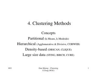
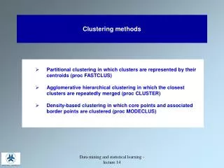
Clustering Techniques Examples of Clustering Techniques: • Hierarchical Clustering: Clusters created from previously established clusters (Agglomerative and Divisive). • K-means: Each cluster is represented by the center of the cluster. • K-medoids: Each cluster is represented by one of the objects in the cluster. • Affinity Propagation: Clustering by “passing messages” between data points.
Two Types of Clustering Techniques • Partitional algorithms: Construct various partitions and then evaluate them by some criterion (ex. k-means, k-medoids). • Hierarchical algorithms: Create a hierarchical decomposition of the set of objects using some criterion. Hierarchical Partitional
Hierarchical Clustering • Clusters created from previously established clusters. • This method builds the hierarchy from the individual elements by progressively merging clusters. • Two types of Hierarchical Clustering: Agglomerative (“bottom-up) and Divisive (“top-down”). • Agglomerative: begin with each element as a separate cluster and merge them into successively larger clusters • Divisive: begin with the whole set and proceed to divide it into successively smaller clusters.
G1 G6 G6 G5 G1 G2 G5 G2 G3 G4 G3 G4 Example of Agglomerative Hierarchical Clustering
Another (more lighthearted) Example of Agglomerative Hierarchical Clustering Choose the best … Choose the best … Choose the best …
Advantages/Disadvantages to Hierarchical Clustering Advantages: • No need to specify the number of clusters in advance. • Generates smaller clusters which may be helpful for discovery. Disadvantages: • Objects may be 'incorrectly' grouped at an early stage. The result should be examined closely to ensure it makes sense. • Use of different distance metrics for measuring distances between clusters may generate different results. • Interpretation of results is subjective.
Partitional Algorithms: K-means and K-medoids • Partitioning Method: Construct a partition of a database D of n objects into a set of k clusters. • Given a k, find a partition of k clusters that optimizes the chosen partitioning criterion. • Whereas Hierarchical Algorithms find successive clusters using previously established clusters, Partitional algorithms determine all clusters at once.
K-means and K-medoids • Both attempt to minimize squared error, the distance between points labeled to be in a cluster and a point designated as the center of that cluster.
K-means Clustering - Each cluster is represented by the center of the cluster. The algorithm steps: Step 1: Choose the number of clusters, k. Step 2: Randomly generate k clusters and determine the cluster centers, or directly generate k random points as cluster centers. Step 3: Assign each point to the nearest cluster center. Step 4: Recompute the new cluster centers. Step 5: Repeat the two previous steps until some convergence criterion is met (usually that the assignment hasn't changed).
k3 k1 k2 Step 1: Choose the number of clusters, k. Algorithm: k-means, Distance Metric: Euclidean Distance 5 4 3 2 1 0 0 1 2 3 4 5
k1 k2 k3 Step 2: Randomly generate k clusters and determine the cluster centers, or directly generate k random points as cluster centers. 5 4 3 2 1 0 0 1 2 3 4 5
k1 k2 k3 Step 3: Assign each point to the nearest cluster center. 5 4 3 2 1 0 0 1 2 3 4 5
k1 k2 k3 Step 4: Recompute the new cluster centers. 5 4 3 2 1 0 0 1 2 3 4 5
k1 k2 k3 Step 5: Repeat the two previous steps until some convergence criterion is met
Advantages/Disadvantages to K-means technique Advantages: • Relatively efficient Disadvantages: • Unable to handle noisy data and outliers • Very sensitive with respect to initial choice of clusters • Need to specify number of clusters in advance • Applicable only when mean is defined – what about categorical data?
K-medoids Clustering • Each center is represented by one of the objects (representative objects, called medoids) in the cluster. 1) The algorithm begins with arbitrary selection of the k objects as medoid points out of n data points (n>k) 2) After selection of the k medoid points, associate each data object in the given data set to most similar medoid. 3) Randomly select nonmedoid object O’ 4) compute total cost , S of swapping initial medoid object to O’ 5) If S<0, then swap initial medoid with the new one ( if S<0 then there will be new set of medoids) 6) repeat steps 2 to 5 untill there is change in the medoid.
Step 1-2:Choose k=2.Choose C1=(3,4) and C2=(7,4) as the medoids.Calculate the distance so as to associate each data object to its nearest medoid.
Step 3-6: - Randomly select nonmedoid object O’- Compare efficiency of O’ as a medoid to original O and swap if necessary- Repeat until there is no change in the medoid(in this case – bad idea!)
Advantages/Disadvantages to k-medoid technique Advantages: • Relatively efficient • Better at handling noise and outliers than k-means Disadvantages: • Need to specify number of clusters in advance • Slower than k-means
Affinity Propagation • Clustering by “passing messages” between data points (Frey and Dueck, 2007). • Innovative clustering technique that purports to combine the advantages of affinity-based clustering and model-based clustering. • Similar to k-medoid clustering in that representative data points called “exemplars” used as centers to clusters. • However, more efficient than k-medoid in the sense that the exemplars are not chosen randomly. The initial choice is close to a good solution.
Input • Negative Euclidean distance used to measure similarity. • Number of original clusters do NOT have to be specified. • Takes as an input real valued similarities between data points. Similarity s(i,k) shows how well the data point with index k is suited to be the exemplar for data point i. • Takes into account a real number s(k,k) for each data point k so that data points with larger values of s(k,k) are more likely to be chosen as exemplars.
Messages • Two kinds of messages exchanged between data points: • “responsibility” r(i,k) is sent from data point i → candidate exemplar point k Indicates how strongly each data point favors the candidate exemplar over other candidate exemplars. 2. “availability” a(i,k) is sent from candidate exemplar point k → data point i Indicates to what degree each candidate exemplar is available as a cluster center for the data point.
Responsibilities • Initially, availabilities are initialized to zero: a(i,k) = 0 • Responsibilities computed as Availabilities will eventually drop below zero as points are assigned to other exemplars. Will decrease the effective values of the input similarities, removing candidate exemplars from competition. Lets all candidate exemplars compete for ownership of a data point.
Availabilities Availabilities set to self-responsibility plus r(k,k) plus the sum of the positive responsibilities candidate exemplar k receives from other points. Self-availability a(k,k) reflects evidence that k is an exemplar based on positive responsibilities sent to candidate exemplar k from other points.