Download
1 / 57
570 likes | 588 Views
Learn about automated discovery and unsupervised clustering methods, including K-Means and Kohonen SOM, for segmenting data and predicting trends. Understand clustering techniques and their applications in market segmentation.

E N D
COMP3503 Automated Discovery andClustering Methods Daniel L. Silver
Agenda • Automated Exploration/Discovery (unsupervised clustering methods) • K-Means Clustering Method • Kohonen Self Organizing Maps (SOM)
x2 x1 f(x) x Overview of Modeling Methods A • Automated Exploration/Discovery • e.g.. discovering new market segments • distance and probabilistic clustering algorithms • Prediction/Classification • e.g.. forecasting gross sales given current factors • statistics (regression, K-nearest neighbour) • artificial neural networks, genetic algorithms • Explanation/Description • e.g.. characterizing customers by demographics • inductive decision trees/rules • rough sets, Bayesian belief nets B if age > 35 and income < $35k then ...
Automated Exploration/DiscoveryThrough Unsupervised Learning Objective: To induce a model without use of a target (supervisory) variable such that similar examples are grouped into self-organized clusters or catagories. This can be considered a method of unsupervised concept learning. There is no explicit teaching signal. C A B x2 x1
Classification Systems and Inductive Learning Basic Framework for Inductive Learning Environment Testing Examples THIS FRAMEWORK IS NOTAPPLICABLE TO UNSUPERVISED LEARNING Training Examples Induced Model of Classifier Inductive Learning System ~ h(x) = f(x)? (x, f(x)) Output Classification A problem of representation and search for the best hypothesis, h(x). (x, h(x))
Automated Exploration/DiscoveryThrough Unsupervised Learning Multi-dimensional Feature Space Income $ Education Age
Automated Exploration/DiscoveryThrough Unsupervised Learning Common Uses • Market segmentation • Population catagorization • Product/service catagorization • Automated subject indexing (WEBSOM) • Multi-variable (vector) quantization • reduce several variables to one
Clustering techniques apply when there is no class to be predicted Aim: divide instances into “natural” groups Clusters can be: disjoint vs. overlapping deterministic vs. probabilistic flat vs. hierarchical WHF 3.6 & 4.8 Clustering
Representing clusters I Venn diagram Simple 2-D representation Overlapping clusters
Representing clusters II Probabilistic assignment Dendrogram 1 2 3 a 0.4 0.1 0.5 b 0.1 0.8 0.1 c 0.3 0.3 0.4 d 0.1 0.1 0.8 e 0.4 0.2 0.4 f 0.1 0.4 0.5 g 0.7 0.2 0.1 h 0.5 0.4 0.1 … NB: dendron is the Greek word for tree
The classic clustering algorithm -- k-means k-means clusters are disjoint, deterministic, and flat 3.6 & 4.8 Clustering
K-Means Clustering Method • Consider m examples each with 2 attributes [x,y] in a 2D input space • Method depends on storing all examples • Set number of clusters, K • Centroid of clusters is initially the average coordinates of first K examples or randomly chosen coordinates
K-Means Clustering Method • Until cluster boundaries stop changing • Assign each example to the cluster who’s centroid is nearest - using some distance measure (e.g. Euclidean distance) • Recalculate centroid of each cluster: e.g. [mean(x), mean(y)] for all examples currently in cluster K
3.6 & 4.8 Clustering DEMO: http://home.dei.polimi.it/matteucc/Clustering/tutorial_html/AppletKM.html
K-Means Clustering Method • Advantages: • simple algorithm to implement • can form very interesting groupings • clusters can be characterized by attributes / values • sequential learning method • Disadvantages: • all variables must be ordinal in nature • problems transforming categorical variables • requires lots of memory, computation time • does poorly for large numbers of attributes (curse of dimensionality)
Discussion Algorithm minimizes squared distance to cluster centers Result can vary significantly based on initial choice of seeds Can get trapped in local minimum Example: To increase chance of finding global optimum: restart with different random seeds Can we applied recursively with k = 2 initial cluster centres instances
Kohonen SOM (Self Organizing Feature Map) • Implements a version of K-Means • Two layer feed-forward neural network • Input layer fully connected to an output layer of N outputs arranged in 2D; weights initialized to small random values • Objective is to arrange the outputs into a map which is topologically organized according to the features presented in the data
Kohonen SOM The Training Algorithm • Present an example to the inputs • The winning output is that whose weights are “closest” to the input values (e.g. Euclidean dist.) • Adjust the winners weights slightly to make it more like the example • Adjust the weights of the neighbouring output nodes relative to proximity to chosen output node • Reduce the neighbourhood size Repeated for I iterations through examples
SOM Demos • http://www.eee.metu.edu.tr/~alatan/Courses/Demo/Kohonen.htm • http://davis.wpi.edu/~matt/courses/soms/applet.html
Kohonen SOM • In the end, the network effectively quantizes the input vector of each example to a single output node • The weights to that node indicate the feature values that characterize the cluster • Topology of map shows association/ proximity of clusters • Biological justification - evidence of localized topological mapping in neocortex
Faster distance calculations Can we use kD-trees or ball trees to speed up the process? Yes: First, build tree, which remains static, for all the data points At each node, store number of instances and sum of all instances In each iteration, descend tree and find out which cluster each node belongs to Can stop descending as soon as we find out that a node belongs entirely to a particular cluster Use statistics stored at the nodes to compute new cluster centers
6.8 Clustering: how many clusters? How to choose k in k-means? Possibilities: Choose k that minimizes cross-validated squared distance to cluster centers Use penalized squared distance on the training data (eg. using an MDL criterion) Apply k-means recursively with k = 2 and use stopping criterion (eg. based on MDL) Seeds for subclusters can be chosen by seeding along direction of greatest variance in cluster(one standard deviation away in each direction from cluster center of parent cluster) Implemented in algorithm called X-means (using Bayesian Information Criterion instead of MDL)
Hierarchical clustering Recursively splitting clusters produces a hierarchy that can be represented as a dendogram Could also be represented as a Venn diagram of sets and subsets (without intersections) Height of each node in the dendogram can be made proportional to the dissimilarity between its children
Agglomerative clustering Bottom-up approach Simple algorithm Requires a distance/similarity measure Start by considering each instance to be a cluster Find the two closest clusters and merge them Continue merging until only one cluster is left The record of mergings forms a hierarchical clustering structure – a binary dendogram
Distance measures Single-linkage Minimum distance between the two clusters Distance between the clusters closest two members Can be sensitive to outliers Complete-linkage Maximum distance between the two clusters Two clusters are considered close only if all instances in their union are relatively similar Also sensitive to outliers Seeks compact clusters
Distance measures cont. Compromise between the extremes of minimum and maximum distance Represent clusters by their centroid, and use distance between centroids – centroid linkage Works well for instances in multidimensional Euclidean space Not so good if all we have is pairwise similarity between instances Calculate average distance between each pair of members of the two clusters – average-linkage Technical deficiency of both: results depend on the numerical scale on which distances are measured
More distance measures Group-average clustering Uses the average distance between all members of the merged cluster Differs from average-linkage because it includes pairs from the same original cluster Ward's clustering method Calculates the increase in the sum of squares of the distances of the instances from the centroid before and after fusing two clusters Minimize the increase in this squared distance at each clustering step All measures will produce the same result if the clusters are compact and well separated
Example hierarchical clustering 50 examples of different creatures from the zoo data Complete-linkage Dendogram Polar plot
Example hierarchical clustering 2 Single-linkage
Incremental clustering Heuristic approach (COBWEB/CLASSIT) Form a hierarchy of clusters incrementally Start: tree consists of empty root node Then: add instances one by one update tree appropriately at each stage to update, find the right leaf for an instance May involve restructuring the tree Base update decisions on category utility
Clustering weather data 1 ID Outlook Temp. Humidity Windy A Sunny Hot High False B Sunny Hot High True C Overcast Hot High False D Rainy Mild High False 2 E Rainy Cool Normal False F Rainy Cool Normal True G Overcast Cool Normal True H Sunny Mild High False I Sunny Cool Normal False J Rainy Mild Normal False 3 K Sunny Mild Normal True L Overcast Mild High True M Overcast Hot Normal False N Rainy Mild High True
Clustering weather data 4 ID Outlook Temp. Humidity Windy A Sunny Hot High False B Sunny Hot High True C Overcast Hot High False D Rainy Mild High False 5 E Rainy Cool Normal False F Rainy Cool Normal True G Overcast Cool Normal True Merge best host and runner-up H Sunny Mild High False I Sunny Cool Normal False J Rainy Mild Normal False 3 K Sunny Mild Normal True L Overcast Mild High True M Overcast Hot Normal False N Rainy Mild High True Consider splitting the best host if merging doesn’t help
Category utility Category utility: quadratic loss functiondefined on conditional probabilities: Every instance in different category numerator becomes maximum number of attributes
Probability-based clustering Problems with heuristic approach: Division by k? Order of examples? Are restructuring operations sufficient? Is result at least local minimum of category utility? Probabilistic perspective seek the most likely clusters given the data Also: instance belongs to a particular cluster with a certain probability
Finite mixtures Model data using a mixture of distributions One cluster, one distribution governs probabilities of attribute values in that cluster Finite mixtures : finite number of clusters Individual distributions are normal (Gaussian) Combine distributions using cluster weights
Two-class mixture model B 62A 47A 52B 64A 51B 65A 48A 49 A 46 B 64A 51A 52B 62A 49A 48B 62A 43A 40 A 48B 64A 51B 63A 43B 65B 66 B 65A 46 A 39B 62B 64A 52B 63B 64A 48B 64A 48 A 51A 48B 64A 42A 48A 41 A 51A 43B 62B 64A 45A 42A 46A 45A 45 data model A=50, A =5, pA=0.6 B=65, B =2, pB=0.4
Learning the clusters Assume: we know there are k clusters Learn the clusters determine their parameters I.e. means and standard deviations Performance criterion: probability of training data given the clusters EM algorithm finds a local maximum of the likelihood
EM algorithm EM = Expectation-Maximization Generalize k-means to probabilistic setting Iterative procedure: E “expectation” step: Calculate cluster probability for each instance M “maximization” step: Estimate distribution parameters from cluster probabilities Store cluster probabilities as instance weights Stop when improvement is negligible
More on EM Estimate parameters from weighted instances Stop when log-likelihood saturates Log-likelihood:
Extending the mixture model More then two distributions: easy Several attributes: easy—assuming independence! Correlated attributes: difficult Joint model: bivariate normal distributionwith a (symmetric) covariance matrix n attributes: need to estimate n + n (n+1)/2 parameters
More mixture model extensions Nominal attributes: easy if independent Correlated nominal attributes: difficult Two correlated attributes v1 v2 parameters Missing values: easy Can use other distributions than normal: “log-normal” if predetermined minimum is given “log-odds” if bounded from above and below Poisson for attributes that are integer counts Use cross-validation to estimate k !
Bayesian clustering Problem: many parameters EM overfits Bayesian approach : give every parameter a prior probability distribution Incorporate prior into overall likelihood figure Penalizes introduction of parameters Eg: Laplace estimator for nominal attributes Can also have prior on number of clusters! Implementation: NASA’s AUTOCLASS
Discussion Can interpret clusters by using supervised learning post-processing step Decrease dependence between attributes? pre-processing step E.g. use principal component analysis Can be used to fill in missing values Key advantage of probabilistic clustering: Can estimate likelihood of data Use it to compare different models objectively
WEKA Tutroial K-means, EM and Cobweb and the Weather data http://www.cs.ccsu.edu/~markov/ccsu_courses/DataMining-Ex3.html