Download
1 / 18
180 likes | 346 Views
Component Modelling. The interaction between conservation equations and equations describing the physical process going on internally in a component. Black box model. Only offers information about the thermodynamic conditions at inlet and outlet from a given component.

E N D
Component Modelling • The interaction between conservation equations and • equations describing the physical process going on • internally in a component. Analysis, Modelling and Simulation of Energy Systems, SEE-T9 Mads Pagh Nielsen
Black box model Only offers information about the thermodynamic conditions at inlet and outlet from a given component. At stationary modelling start up phenomena and transients caused by alternating loads are not considered and thus knowledge about the internal process going on in the components is redundant. Analysis, Modelling and Simulation of Energy Systems, SEE-T9 Mads Pagh Nielsen
Energy- and mass conservation Analysis, Modelling and Simulation of Energy Systems, SEE-T9 Mads Pagh Nielsen
System boundaries • Setting up conservation equations: • Two-gate approach versus multigate approach: • Two-gate method: Multigate method Multiple in- and outputs One input & one output ? ? 2 components 1component Analysis, Modelling and Simulation of Energy Systems, SEE-T9 Mads Pagh Nielsen
Example: Pump + • Inlet conditions: h, p, T and . T is calculated as a function of pressure and enthalpy. • Besides that, either Wpump or the desired exit pressure p2 should be given. • Physical property: pump Analysis, Modelling and Simulation of Energy Systems, SEE-T9 Mads Pagh Nielsen
Example: Air compressor Analysis, Modelling and Simulation of Energy Systems, SEE-T9 Mads Pagh Nielsen
Example: Heat exchanger Analysis, Modelling and Simulation of Energy Systems, SEE-T9 Mads Pagh Nielsen
LMTD-method Analysis, Modelling and Simulation of Energy Systems, SEE-T9 Mads Pagh Nielsen
Typical U-values: Pre-heater ~ 34 W/(m²·K) Evaporator ~ 80 W/(m²·K) Super heater ~ 72 W/(m²·K) Water-Water ~ 1500 (800-2500) W/(m²·K) Analysis, Modelling and Simulation of Energy Systems, SEE-T9 Mads Pagh Nielsen
Example: Gas engine Conservation of energy: Continuity: Analysis, Modelling and Simulation of Energy Systems, SEE-T9 Mads Pagh Nielsen
Efficiency characteristic Analysis, Modelling and Simulation of Energy Systems, SEE-T9 Mads Pagh Nielsen
Exhaust temperature Analysis, Modelling and Simulation of Energy Systems, SEE-T9 Mads Pagh Nielsen
Cooling efficiency Analysis, Modelling and Simulation of Energy Systems, SEE-T9 Mads Pagh Nielsen
Exhaust massflow Analysis, Modelling and Simulation of Energy Systems, SEE-T9 Mads Pagh Nielsen
{/////////////////////////////////////////////////////} { Gas engine } {/////////////////////////////////////////////////////} R[1]=0.6{Relative hum. of inlet air} f[1]=humrat(AirH2o, p=p[1], h=h[1], R=R[1]) Load=100 {Full load} H_combustion[1]=49.5e6{Lower heating value of natural gas} Eta_generator=0.95 {Efficiency of generator} Q[4]=m[2]*H_combustion {Stoichiometric combustion} Q[6]=0,04*W[5] {Heat loss from engine} W[5]=Q[4]*Eta_shaft{Shaft power} Q[7]=Q[4]*Eta_cooling{Cooling energy} W[5]=(W_el/Eta_generator){Calculation of electricity produced} W[5]=(Load/100)*Size {Relate shaft power to load} CALL Regressions(Size;Load:T_exh[3];m_dot_exh[3];Eta_cooling;Eta_shaft) Equations: Analysis, Modelling and Simulation of Energy Systems, SEE-T9 Mads Pagh Nielsen
Regressions for gas engine: PROCEDURE Reg(Motorstr;Last:T; m;Eta_varme;Eta_aksel) IF Motorstr<=1,5 THEN {Reg for CATERPILLAR 3500-series (k1-k3)} k1=-1,56758264751006*(Motorstr*Last) : k2=k1+8,36936811270700E-1*(Motorstr^2*Last) k3=k2+-3,42845055730651E-16*(Motorstr*Last^2) : k4=k3+ 2,99266904660311E-16*(Motorstr^2*Last^2) k5=k4+2,84051875454190E2+3,83032124894794E+2*Motorstr : k6=k5+-2,30497204202655E2*Motorstr^2+ 5,59104477611930E-1*Last T:=k6+6,85893399368642E-17*Last^2 k7=-1,14150573395760E-1*(Motorstr*Last) : k8=k7+7,96699062703951E-2*(Motorstr^2*Last) : k9=k8+ 8,36505679102166E-4*(Motorstr*Last^2) k10=k9-5,22119006981289E-4*(Motorstr^2*Last^2) : k11=k10-1,39907903460236+4,28181037738979*Motorstr : k12=k11-2,60141328430843*Motorstr^2+ 4,36490378444878E-2*Last m:=k12-2,86807025546440E-4*Last^2 k13=2,19831291406054E-2*(Motorstr*Last) : k14=k13-1,44163671822562E-2*(Motorstr^2*Last) : k15=k14+-1,60255776666399E-4*(Motorstr*Last^2) k16=k15+1,05717344183216E-4*(Motorstr^2*Last^2) : k17=k16+7,36280756330728E-1-7,62002120553441E-1*Motorstr : k18=k17+4,71623296935500E-1*Motorstr^2-9,32664939348261E-3*Last Eta_varme:=k18 +6,12378936776826E-5*Last^2 k19=-1,99946179007292E-3*(Motorstr*Last) : k20=k19+1,21549137646842E-3*(Motorstr^2*Last) : k21=k20+1,45131112263936E-5*(Motorstr*Last^2) k22=k21-9,50827088959231E-6*(Motorstr^2*Last^2) : k23=k22+1,81239004416123E-1+8,37224175248884E-2*Motorstr : k24=k23-3,05022195543315E-2*Motorstr^2+3,20380803845934E-3*Last : Eta_aksel:=k24-1,55230096707470E-5*Last^2 ELSE {Reg for CATERPILLAR 3600-series} k25=-2,53313202482839E-1*(Motorstr*Last) : k26=k25+5,08354811324176E-2*(Motorstr^2*Last) : k27=k26+2,02650561986270E-3*(Motorstr*Last^2) k28=k27-4,06683849059337E-4*(Motorstr^2*Last^2) : k29=k28+4,40706780944827E2+2,53313202482813E+1*Motorstr : k30=k29-5,08354811324126*Motorstr^2+1,42932190551758E-1*Last T:=k30-1,04234575244140E-2*Last^2 k31=-1,33788890577105E-2*(Motorstr*Last) : k32=k31+3,14987756577728E-3*(Motorstr^2*Last) : k33=k32+3,37507315437329E-4*(Motorstr*Last^2) k34=k33-4,13391073261964E-5*(Motorstr^2*Last^2) : k35=k34-1,79904317687621+9,68662711839557E-1*Motorstr : k36=k35-8,51957284061772E-2*Motorstr^2+6,21466578567492E-2*Last m:=k36-5,94451119750688E-4*Last^2 : k37=3,03270909860921E-3*(Motorstr*Last) : k38=k37-6,30752577079704E-4*(Motorstr^2*Last) k39=k38-1,82497622039065E-5*(Motorstr*Last^2) : k40=k39+3,74291908784650E-6*(Motorstr^2*Last^2) : k41=k40+3,11862476018024E-1+-1,03069392710923E-1*Motorstr : k42=k41+2,22944942660193E-2*Motorstr^2-3,98480909049131E-3*Last Eta_varme:=k42+2,81447180524241E-5*Last^2 k43=-2,33866878272789E-3*(Motorstr*Last) : k44=k43+4,26254234584089E-4*(Motorstr^2*Last) : k45=k44+1,16524914451450E-5*(Motorstr*Last^2) k46=k45-2,19352296721786E-6*(Motorstr^2*Last^2) : k47=k46+1,61524621500911E-1+9,59653427654178E-2*Motorstr :k48=k47-1,60580973780507E-2*Motorstr^2+4,66986417775120E-3*Last Eta_aksel:=k48-1,98706347417594E-5*Last^2 ENDIF END Analysis, Modelling and Simulation of Energy Systems, SEE-T9 Mads Pagh Nielsen
Example: Gas turbine Can be modelled almost like a gas engine. The gas turbine is modelled similarly as an air compressor. Only note that gas turbines are sensitive to pressure drop in boiler! Analysis, Modelling and Simulation of Energy Systems, SEE-T9 Mads Pagh Nielsen
Next time: Analysis, Modelling and Simulation of Energy Systems, SEE-T9 Mads Pagh Nielsen