Download
1 / 32
340 likes | 423 Views
Explore the dynamics of sediment transport in nature including settling velocity, erosion mechanisms, and critical shear calculations. Learn about Hjulström’s curve, sediment transport models, and calculation methods.

E N D
5. Sediment transport models Huttula Lecture Set 4
Settling velocity (vf): Stoke’s equation • Assumption: spherical particles • Gravity force = drag force • Particle reaches a constant settling velocity • This velocituy is dependent on: fluid viscosity (), density difference between the particle and water (s-) and particle diameter (d), • g=gravity constant= 9,81 m/s2 • Velocity range: From 0.07 m/d (clay, d=1.2 m) to 710 m/d (sand, d=200m), density=2.5 gcm-3 Huttula Lecture Set 4
Settling speed in nature • Particles are seldom spherical: clay particles are like plates • Aggregation of particles happens due to the electromagnetic forces cohesive soils (clays, mud…) • Organic compounds like humic substances have a very fragile structure changes even in water column • velocity from Stoke’s equation has to be corrected with empirical relations • Baba& Komar, 1981: vreal=0.761vf • In sediment transport models vf is calculated using the median particle size from a surface sediment sample Huttula Lecture Set 4
Erosion or resuspension from bottom • Acting forces on a particle laying on the bottom • difference between gravity on buoyancy • drag force by the current • lifting force due to the pressure differences as caused by water flowing between particles • electromagnetic forces causing aggregation • Term 1. density difference and particle (diameter)3 • Terms 2 and 3. shear force caused by current and particle (diameter)2 • Shields’s empirical curve for erosion in design of structures • A simplified erosion curve by Hjulström (erosion vs. current velocity) • In models we use most often the critical shear concept Huttula Lecture Set 4
Hjulström’s curve for erosion Huttula Lecture Set 4
Critical shear • Total shear () on the lake bottom = • shear by orbital movements of waves = f(wind fetch over lake, lake mean depth, wind velocity and duration)Materials\Lake Säkylän Pyhäjärvi.pdf • shear by currents • > critical shear (cr), erosion happens with a rate a*(excess shear)b • cr, a and b are experimental values, which we calibrate during model application • values for cr: 0.008…1 Nm-2, b=1..3, a = depends on sediment • In this formulation there is no consolidation effects and bottom morphology included Huttula Lecture Set 4
Calculation of sediment transport • Simple screening tools:http://el.erdc.usace.army.mil/dots/doer/tools.html • Using numerical flow models for predicting the horizontal current field • Suspended solids concentration is calculated with concentration equation • Following terms in concentration equation: • advection with settling speed in vertical dimension • turbulence • mass flow from tributaries and to out flowing river • settling and deposition to bottom • erosion or resuspension from bottom Huttula Lecture Set 4
Example from Mänttä 2DH flow model with BOD7 water quality compartment Sediment was light organic fibre Short term regulation at hydropower plant Huttula Lecture Set 4
Example from Karhijärvi • Three different models were tested 2DH, 2DV and 3D model • Models were tested in an runoff case in Oct 1992, when heavy rains caused erosion from watershed and a heavy suspended solids load to lake • Data: winds on the lake, water current observations, turbidity observations • 3D model gave best results Huttula Lecture Set 4
Mänttä: Transport model resultSediment: fibrous material Huttula Lecture Set 4
Sediment transport in Tanganyika • Model simulation • lake wide circulation model boundary values (current velocity) for high resolution model at river mouths • flow model and suspended sediment transport models • SS input was estimated from historical data • real winds from atmospheric model HIRLAM (this model was used first time in tropics) Huttula Lecture Set 4
3D FLOW MODEL Calculated depth-averaged flow on 24.08.97 04:00. Huttula Lecture Set 4 Calculated depth-averaged flow on 24.08.97 20:00
3D SEDIMENT TRANSPORT MODEL (A), 12:00 24.08.97 (B) 0:00 28.08.97 (C) after 22, 82 and 166 hours after the simulation start respectively. Huttula Lecture Set 4
6. Water quality models Huttula Lecture Set 4
Concentration equation where, • c = concentration, qL= amount of loading release , n= length measure against release, u,v,w = x-, y- ja z- advective velocities in x-, y- ja z- directions, Dx, Dy, Dz = dispersion coefficients, R(T,c) = biogeochemical changes in concentration Huttula Lecture Set 4
Application of WQ-models • We include : • Advection • Dispersion • Settling on the bottom • Bio- chemical processes • Decomposition, respiration, aeration, anaerobic release of P from the bottom • Select the most important variables concerning the problem • Oxygen, nutrients (like P,N), chlorophyll-a and some conservative substance (like Na) • Limiting factors (light, nutrients, …) must be included. Check! • Temperature corrections must be included. Check! Huttula Lecture Set 4
Lake Lappajärvi WQ-model • PROBE temperature model • Materials\Effects of Climate Change....pdf • PROBE-WQ model • Materials\Lappajarvi_WQ.pdf Huttula Lecture Set 4
Oxygen model Huttula Lecture Set 4
Phytoplankton biomass and ToTP Huttula Lecture Set 4
Interactions in EIA-SYKE-model Huttula Lecture Set 4
Other WQ-model applications • Several case studies Materials\Flow_and_WQ_Models_Sarkkula.pdf • Lake Pyhäselkä • Materials\Pyhaselka.pdf • What happened to WQ after real reduction of loads? • Materials\IAWQ99.pdf Huttula Lecture Set 4
Summary of WQ-model calculations • Check that you have data to describe WQ in variable discharge and loading conditions • Select those properties (variables), which describe best the effects of loading and concentrate calibration on them • Use most simple parameterization of the variables • First coefficient values from literature and by experience • Compare the calculated and observed values • Select the conditions (weather, discharge and loading) during which the effects are described ….and run the model!! Huttula Lecture Set 4