Download
1 / 54
540 likes | 736 Views
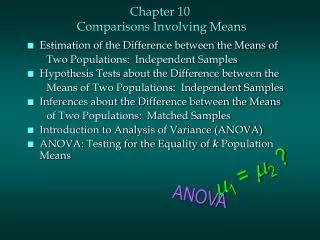
1 = 2 ?. ANOVA. Chapter 10 Comparisons Involving Means. Estimation of the Difference between the Means of Two Populations: Independent Samples Hypothesis Tests about the Difference between the Means of Two Populations: Independent Samples

E N D
1 = 2 ? ANOVA Chapter 10 Comparisons Involving Means • Estimation of the Difference between the Means of Two Populations: Independent Samples • Hypothesis Tests about the Difference between the Means of Two Populations: Independent Samples • Inferences about the Difference between the Means of Two Populations: Matched Samples • Introduction to Analysis of Variance (ANOVA) • ANOVA: Testing for the Equality of k Population Means
Estimation of the Difference Between the Means of Two Populations: Independent Samples • Point Estimator of the Difference between the Means of Two Populations • Sampling Distribution • Interval Estimate of Large-Sample Case • Interval Estimate of Small-Sample Case
Point Estimator of the Difference Betweenthe Means of Two Populations • Let 1 equal the mean of population 1 and 2 equal the mean of population 2. • The difference between the two population means is 1 - 2. • To estimate 1 - 2, we will select a simple random sample of size n1 from population 1 and a simple random sample of size n2 from population 2. • Let equal the mean of sample 1 and equal the mean of sample 2. • The point estimator of the difference between the means of the populations 1 and 2 is .
Sampling Distribution of • Properties of the Sampling Distribution of • Expected Value
Sampling Distribution of • Properties of the Sampling Distribution of • Standard Deviation where: 1 = standard deviation of population 1 2 = standard deviation of population 2 n1 = sample size from population 1 n2 = sample size from population 2
Interval Estimate of 1 - 2:Large-Sample Case (n1> 30 and n2> 30) • Interval Estimate with 1 and 2 Known where: 1 - is the confidence coefficient
Interval Estimate of 1 - 2:Large-Sample Case (n1> 30 and n2> 30) • Interval Estimate with 1 and 2 Unknown where:
Example: Par, Inc. • Interval Estimate of 1 - 2: Large-Sample Case Par, Inc. is a manufacturer of golf equipment and has developed a new golf ball that has been designed to provide “extra distance.” In a test of driving distance using a mechanical driving device, a sample of Par golf balls was compared with a sample of golf balls made by Rap, Ltd., a competitor. The sample statistics appear on the next slide.
Example: Par, Inc. • Interval Estimate of 1 - 2: Large-Sample Case • Sample Statistics Sample #1 Sample #2 Par, Inc. Rap, Ltd. Sample Size n1 = 120 balls n2 = 80 balls Mean = 235 yards = 218 yards Standard Dev. s1 = 15 yards s2 = 20 yards
Example: Par, Inc. • Point Estimate of the Difference Between Two Population Means 1 = mean distance for the population of Par, Inc. golf balls 2 = mean distance for the population of Rap, Ltd. golf balls Point estimate of 1 - 2 = = 235 - 218 = 17 yards.
Simple random sample of n1 Par golf balls x1 = sample mean distance for sample of Par golf ball Simple random sample of n2 Rap golf balls x2 = sample mean distance for sample of Rap golf ball x1 - x2 = Point Estimate of m1 –m2 Point Estimator of the Difference Betweenthe Means of Two Populations Population 1 Par, Inc. Golf Balls m1 = mean driving distance of Par golf balls Population 2 Rap, Ltd. Golf Balls m2 = mean driving distance of Rap golf balls m1 –m2= difference between the mean distances
Example: Par, Inc. • 95% Confidence Interval Estimate of the Difference Between Two Population Means: Large-Sample Case, 1 and 2 Unknown Substituting the sample standard deviations for the population standard deviation: = 17 + 5.14 or 11.86 yards to 22.14 yards. We are 95% confident that the difference between the mean driving distances of Par, Inc. balls and Rap, Ltd. balls lies in the interval of 11.86 to 22.14 yards.
Interval Estimate of 1 - 2:Small-Sample Case (n1 < 30 and/or n2 < 30) • Interval Estimate with 2 Known where:
Interval Estimate of 1 - 2:Small-Sample Case (n1 < 30 and/or n2 < 30) • Interval Estimate with 2 Unknown where:
Example: Specific Motors Specific Motors of Detroit has developed a new automobile known as the M car. 12 M cars and 8 J cars (from Japan) were road tested to compare miles-per- gallon (mpg) performance. The sample statistics are: Sample #1 Sample #2 M CarsJ Cars Sample Size n1 = 12 cars n2 = 8 cars Mean = 29.8 mpg = 27.3 mpg Standard Deviation s1 = 2.56 mpg s2 = 1.81 mpg
Example: Specific Motors • Point Estimate of the Difference Between Two Population Means 1 = mean miles-per-gallon for the population of M cars 2 = mean miles-per-gallon for the population of J cars Point estimate of 1 - 2 = = 29.8 - 27.3 = 2.5 mpg.
Example: Specific Motors • 95% Confidence Interval Estimate of the Difference Between Two Population Means: Small-Sample Case We will make the following assumptions: • The miles per gallon rating must be normally distributed for both the M car and the J car. • The variance in the miles per gallon rating must be the same for both the M car and the J car.
Example: Specific Motors • 95% Confidence Interval Estimate of the Difference Between Two Population Means: Small-Sample Case Using the t distribution with n1 + n2 - 2 = 18 degrees • of freedom, the appropriate t value is t.025 = 2.101. • We will use a weighted average of the two sample • variances as the pooled estimator of 2.
Example: Specific Motors • 95% Confidence Interval Estimate of the Difference Between Two Population Means: Small-Sample Case = 2.5 + 2.2 or .3 to 4.7 miles per gallon. We are 95% confident that the difference between the mean mpg ratings of the two car types is from .3 to 4.7 mpg (with the M car having the higher mpg).
Hypothesis Tests About the Difference between the Means of Two Populations: Independent Samples • Hypotheses H0: 1 - 2< 0 H0: 1 - 2> 0 H0: 1 - 2 = 0 Ha: 1 - 2 > 0 Ha: 1 - 2 < 0 Ha: 1 - 2 0 • Test Statistic Large-Sample Small-Sample
Example: Par, Inc. • Hypothesis Tests About the Difference between the Means of Two Populations: Large-Sample Case Par, Inc. is a manufacturer of golf equipment and has developed a new golf ball that has been designed to provide “extra distance.” In a test of driving distance using a mechanical driving device, a sample of Par golf balls was compared with a sample of golf balls made by Rap, Ltd., a competitor. The sample statistics appear on the next slide.
Example: Par, Inc. • Hypothesis Tests About the Difference Between the Means of Two Populations: Large-Sample Case • Sample Statistics Sample #1 Sample #2 Par, Inc. Rap, Ltd. Sample Size n1 = 120 balls n2 = 80 balls Mean = 235 yards = 218 yards Standard Dev. s1 = 15 yards s2 = 20 yards
Example: Par, Inc. • Hypothesis Tests About the Difference Between the Means of Two Populations: Large-Sample Case Can we conclude, using a .01 level of significance, that the mean driving distance of Par, Inc. golf balls is greater than the mean driving distance of Rap, Ltd. golf balls?
Example: Par, Inc. • Hypothesis Tests About the Difference Between the Means of Two Populations: Large-Sample Case 1 = mean distance for the population of Par, Inc. golf balls 2 = mean distance for the population of Rap, Ltd. golf balls • HypothesesH0: 1 - 2< 0 Ha: 1 - 2 > 0
Example: Par, Inc. • Hypothesis Tests About the Difference Between the Means of Two Populations: Large-Sample Case • Rejection Rule Reject H0 if z > 2.33
Example: Par, Inc. • Hypothesis Tests About the Difference Between the Means of Two Populations: Large-Sample Case • Conclusion Reject H0. We are at least 99% confident that the mean driving distance of Par, Inc. golf balls is greater than the mean driving distance of Rap, Ltd. golf balls.
Example: Specific Motors • Hypothesis Tests About the Difference Between the Means of Two Populations: Small-Sample Case Can we conclude, using a .05 level of significance, that the miles-per-gallon (mpg) performance of M cars is greater than the miles-per-gallon performance of J cars?
Example: Specific Motors • Hypothesis Tests About the Difference Between the Means of Two Populations: Small-Sample Case 1 = mean mpg for the population of M cars 2 = mean mpg for the population of J cars • HypothesesH0: 1 - 2< 0 Ha: 1 - 2 > 0
Example: Specific Motors • Hypothesis Tests About the Difference Between the Means of Two Populations: Small-Sample Case • Rejection Rule Reject H0 if t > 1.734 (a = .05, d.f. = 18) • Test Statistic where:
Inference About the Difference between the Means of Two Populations: Matched Samples • With a matched-sample design each sampled item provides a pair of data values. • The matched-sample design can be referred to as blocking. • This design often leads to a smaller sampling error than the independent-sample design because variation between sampled items is eliminated as a source of sampling error.
Example: Express Deliveries • Inference About the Difference between the Means of Two Populations: Matched Samples A Chicago-based firm has documents that must be quickly distributed to district offices throughout the U.S. The firm must decide between two delivery services, UPX (United Parcel Express) and INTEX (International Express), to transport its documents. In testing the delivery times of the two services, the firm sent two reports to a random sample of ten district offices with one report carried by UPX and the other report carried by INTEX. Do the data that follow indicate a difference in mean delivery times for the two services?
Example: Express Deliveries Delivery Time (Hours) District OfficeUPXINTEXDifference Seattle 32 25 7 Los Angeles 30 24 6 Boston 19 15 4 Cleveland 16 15 1 New York 15 13 2 Houston 18 15 3 Atlanta 14 15 -1 St. Louis 10 8 2 Milwaukee 7 9 -2 Denver 16 11 5
Example: Express Deliveries • Inference About the Difference between the Means of Two Populations: Matched Samples Let d = the mean of the difference values for the two delivery services for the population of district offices • Hypotheses H0: d = 0, Ha: d
Example: Express Deliveries • Inference About the Difference between the Means of Two Populations: Matched Samples • Rejection Rule • Assuming the population of difference values is approximately normally distributed, the t distribution with n - 1 degrees of freedom applies. With = .05, t.025 = 2.262 (9 degrees of freedom). • Reject H0 if t < -2.262 or if t > 2.262
Example: Express Deliveries • Inference About the Difference between the Means of Two Populations: Matched Samples
Example: Express Deliveries • Inference About the Difference between the Means of Two Populations: Matched Samples • Conclusion • Reject H0. • There is a significant difference between the mean delivery times for the two services.
Introduction to Analysis of Variance • Analysis of Variance (ANOVA) can be used to test for the equality of three or more population means using data obtained from observational or experimental studies. • We want to use the sample results to test the following hypotheses. H0: 1=2=3=. . . = k Ha: Not all population means are equal
Introduction to Analysis of Variance • If H0 is rejected, we cannot conclude that all population means are different. • Rejecting H0 means that at least two population means have different values.
Assumptions for Analysis of Variance • For each population, the response variable is normally distributed. • The variance of the response variable, denoted 2, is the same for all of the populations. • The observations must be independent.
Analysis of Variance:Testing for the Equality of k Population Means • Between-Treatments Estimate of Population Variance • Within-Treatments Estimate of Population Variance • Comparing the Variance Estimates: The F Test • The ANOVA Table
Between-Treatments Estimateof Population Variance • A between-treatment estimate of 2 is called the mean square treatment and is denoted MSTR. • The numerator of MSTR is called the sum of squares treatment and is denoted SSTR. • The denominator of MSTR represents the degrees of freedom associated with SSTR.
Within-Samples Estimateof Population Variance • The estimate of 2 based on the variation of the sample observations within each sample is called the mean square error and is denoted by MSE. • The numerator of MSE is called the sum of squares error and is denoted by SSE. • The denominator of MSE represents the degrees of freedom associated with SSE.
Comparing the Variance Estimates: The F Test • If the null hypothesis is true and the ANOVA assumptions are valid, the sampling distribution of MSTR/MSE is an F distribution with MSTR d.f. equal to k - 1 and MSE d.f. equal to nT - k. • If the means of the k populations are not equal, the value of MSTR/MSE will be inflated because MSTR overestimates 2. • Hence, we will reject H0 if the resulting value of MSTR/MSE appears to be too large to have been selected at random from the appropriate F distribution.
Test for the Equality of k Population Means • Hypotheses H0: 1=2=3=. . . = k Ha: Not all population means are equal • Test Statistic F = MSTR/MSE • Rejection Rule Reject H0 if F > F where the value of F is based on an F distribution with k - 1 numerator degrees of freedom and nT - 1 denominator degrees of freedom.
Sampling Distribution of MSTR/MSE • The figure below shows the rejection region associated with a level of significance equal to where F denotes the critical value. Do Not Reject H0 Reject H0 MSTR/MSE F Critical Value
ANOVA Table Source of Sum of Degrees of Mean Variation Squares Freedom Squares F TreatmentSSTR k - 1 MSTR MSTR/MSE Error SSE nT - k MSE TotalSST nT - 1 SST divided by its degrees of freedom nT - 1 is simply the overall sample variance that would be obtained if we treated the entire nT observations as one data set.
Example: Reed Manufacturing • Analysis of Variance J. R. Reed would like to know if the mean number of hours worked per week is the same for the department managers at her three manufacturing plants (Buffalo, Pittsburgh, and Detroit). A simple random sample of 5 managers from each of the three plants was taken and the number of hours worked by each manager for the previous week is shown on the next slide.
Example: Reed Manufacturing • Analysis of Variance Plant 1 Plant 2 Plant 3 ObservationBuffaloPittsburghDetroit 1 48 73 51 2 54 63 63 3 57 66 61 4 54 64 54 5 62 74 56 Sample Mean 55 68 57 Sample Variance26.0 26.5 24.5
Example: Reed Manufacturing • Analysis of Variance • Hypotheses H0: 1=2=3 Ha: Not all the means are equal where: 1 = mean number of hours worked per week by the managers at Plant 1 2 = mean number of hours worked per week by the managers at Plant 2 3 = mean number of hours worked per week by the managers at Plant 3
Example: Reed Manufacturing • Analysis of Variance • Mean Square Treatment Since the sample sizes are all equal x = (55 + 68 + 57)/3 = 60 SSTR = 5(55 - 60)2 + 5(68 - 60)2 + 5(57 - 60)2 = 490 MSTR = 490/(3 - 1) = 245 • Mean Square Error SSE = 4(26.0) + 4(26.5) + 4(24.5) = 308 MSE = 308/(15 - 3) = 25.667 =