Why statistics ?
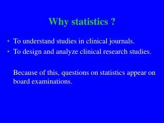
Why statistics ?. To understand studies in clinical journals. To design and analyze clinical research studies. Because of this, questions on statistics appear on board examinations. Types of Clinical Research Studies.

Why statistics ?
E N D
Presentation Transcript
Why statistics ? • To understand studies in clinical journals. • To design and analyze clinical research studies. Because of this, questions on statistics appear on board examinations.
Types of Clinical Research Studies • Cohort: all patients have some condition or something in common (e.g., healthy and living in Framingham, MA) • Case-Control: cases have some condition; controls do not • Randomized, placebo-controlled treatment trial: all patients have the condition • May be unblinded, single blinded or double blinded • Randomized, active-treatment controlled trial: all patients have the condition • often phase 3 trial • Meta analysis: multiple studies of same condition, although definition of the condition may vary from study to study
CONTINUOUS AGE BP CRP AST, CK, glucose, etc HEIGHT WEIGHT BMI Etc. CATEGORICAL GENDER OBESE CURE MI RACE OLD vs YOUNG Etc. Types of Variables
Between subject variability: Serum [Na+] in 135 normals Mean, 140; median 140; range, 135-145 mM; standard deviation2
Basic Statistical Terms • Range: the two extreme values (min and max) • Mean: the average value (uses all values) • Median: the middle value (ignores extreme values), which divides population into two subgroups • Quartiles: divides all values into 4 groups • Tertiles, Quintiles, Percentiles • Standard deviation: measure degrees of difference among all values (uses all values) SD= ((differences from the mean2 )/n-1)
Is there a volunteer ? • /n-1= x/2=? ? = ? SD = ? Mean ± SD = ?
The normal (bell-shaped) distribution • Imagine 2 curves with the same mean, but different SDs ( one wider and less precise; the other narrow-er and more precise). • Now imagine two curves with different means and standard deviations from this curve • Statistical tests are designed to tell us to what extent these different curves could have occurred by chance mean n Standard deviations (SD) from the mean. 95% of values are within 1.96 SD of mean
Some important statistical concepts • Confidence intervals (usually reported as 95% CI) • Number needed to treat (or harm) • Absolute and relative risk or benefit reductions (or increases) • 2-by-2 tables (Chi square, Fisher exact, Mantel Haenszel, others) • Odds or hazard ratios • Type 1 and 2 errors • Estimating sample size needed for a study • Pre- and post-test probabilities and likelihood ratios Ann Int Med 2009: 150: JC6-16
95% CI H. pylori eradication/NSAID study with outcomeof ulcer or no ulcer (categorical outcome): 5 of 51 (10%, or .10) Hp+ pts. who received antibiotics got ulcers when exposed to NSAID. … and 15 of 49 (31%, or .31) Hp+ pts. who did not receive antibiotics got ulcers when exposed to NSAID. What is the chance this difference in outcome occurred due to chance and not the antibiotics? Lancet 2002; 359:9-13.
95% CIs The proportions, p1 and p2, of patients who got ulcers in the 2 groups are an estimate of the true rate. However, from this estimate we can be 95% confident that the actual rates ranges from A to B, with p1 and p2 in the center of the interval from A to B. A and B are the 95% confidence intervals. p1 A B T H E 9 5 % C O N F I D E N C E I N T E R V A L
95% Confidence interval (CI) To calculate the 95% CI for p (i.e., A and B), use this formula: p ± 1.96 [(p)(1-p)/n] The larger the n, which is in the denominator, the smaller (more precise) the CI
5 of 51 (p1=10%, or .10) of the antibiotic group got ulcers when exposed to NSAID for a fixed time • 95% CI =.10 1.96(.1)(.9)/51=.10±.08=[.02, .18] [2%,18%] 15 of 49 (p2=31%, or .31) of the placebo- group got ulcers when exposed to NSAID for a fixed time • 95%CI =.311.96(.31)(.69)/49 =.31±.13=[.18,.44][18%, 44%] Note: the two 95% CIs do not overlap, which means that differences are unlikely to be due to chance. But is the ARR significant?
Absolute risk reduction (ARR) and its 95% CI • The ARR with antibiotics was 31% minus 10%, or 21%. • The 95% CI of the ARR = 21% 1.96 (p1)(1-p1)/n1+(p2)(1-p2)/n2)= 21% 15%, or [6%, 36%]. • The ARR with antibiotics is somewhere between 6% and 36%, with 95% confidence. • This CI does not overlap zero and thus is unlikely due to chance.
Number needed to treat (NNT) • If Absolute Risk reduction (ARR) = 31%-10%=21%, the number needed to treat = 1/ARR = 1/.21=5. • Number needed to harm is the same concept as number needed to treat except that the intervention caused harm rather than good • e.g.: how many patients needed to be treated with antibiotics to produce one drug rash
RRR • Relative Risk Reduction (RRR) = ARR/risk with placebo.. • In this example, RRR= 21%/31% = 68%. • Treat 1,000 pts. with NSAID 310 ulcers (31%) • Treat 1,000 pts. with NSAID + Abs 100 ulcers (10%) • Antibiotic use prevented 210 ulcers (210/310 = 68% = RRR) • Antibiotic use reduced ulcers from 310 to 100, or to 32% of expected, a reduction of 68%. • Note: Length of exposure to NSAID in this study in the 2 groups was identical. If two groups are not followed for an identical time, often the case in trials, outcomes may be higher in the group followed longer and thus events need to be expressed per unit of time (e.g., events per 100 patient-years)
Another example, with the outcome of VTE or no VTE (categorical outcome) 14 of 255 (p1=5.5%, or .055) patients with VTE switched to low-intensity warfarin developed another VTE • 95% CI = [2.6%, 8.4%] … and 37 of 253 (p2=14.6%, or .146) switched to placebo developed another VTE • 95% CI = [10.3%, 18.9%] Could this difference be due to chance? Is this difference likely to be due to chance? Homework: What is ARR and its 95%CI, the RRR, and NNT? New Engl. J. Med. 2003; 348: 1425-1434
Chi Square/Fisher Exact Tests (used for categorical outcomes) • A new treatment for colitis is compared to the standard treatment in 245 patients. • 120 patients are randomized to the new treatment and 125 to the standard treatment. • 90 given the new treatment group go into remission (75%) and 30 (25%) do not. • 75 given the standard treatment go into remission (60%) and 50 (40%) do not. • Is this a significant improvement in outcome, or to what extent could this have been due to chance? Let’s vote!
Step 1: standard 2X2 table New Rx a b a+b Standard Rx c d c+d a + c b + d a+b+c+d=n=total patients in study REMIT NO REMIT
Enter the data from our study New Rx: 90(a) 30(b) 120(a+b) Standard Rx: 75(c) 50(d) 125(c+d) 165 80 245(a+b+c+d)=n REMIT NO REMIT (a+c) (b+d)
Calculate chi square (2) by plugging in numbers into handheld or online calculator 2 = n (ad-bc- n/2)2 (a+b)(c+d)(a+c)(b+d) 2 = 6.264 (p=0.0123) http://www.graphpad.com/quickcalcs/index.cfm Fisher exact test, p=0.0143
We could also have calculated the odds ratio for a remission : New Rx a=90 b=30 Standard Rx c= 75 d=50 odds ratio = ad/bc odds ratio = 4,500/ 2,250= 2 But this odds ratio of 2 could have occurred by chance. We can calculate the 95% CI of the odds ratio to see if the CI overlaps 1 or not. If not, it favors the new treatment with >95% confidence.
95% CI of an odds ratio ln 95% CI = ln OR 1.96 1/a+1/b+1/c+1/d= The OR = 2.00, and so the ln 2.00= 0.693 Thus ln 95% CI= 0.693 0.508 = 0.185, 1.201. To find the CI, we need the antiln of 0.185 and of 1.201. Antiln 0.185 = e.185 =1.20 and antiln 1.201 = e1.201 =3.32. 95% CI =1.20, 3.32. Thus, the odds ratio for a remission with the new treatment is 2.00 (95% CI= 1.20, 3.32). As this odds ratio does not cross 1.00, the difference is unlikely due to chance and is significant at the 0.05 level. e2.72
Type 1 and 2 Errors Null Hypothesis: no differences in 2 treatments Reject null hypothesis Accept null hypothesis Correct decision (no error) Error Correct decision (no error) Error Type 1 () Type 2 ()
Choosing and • (or p) is conventionally set at 0.05 (5%), the chance of a type 1 error if the null hypothesis is rejected ( 5%) • Can state “p<0.05” or give exact p value (e.g., p=0.01) • is often set at 2 to 4 times , or 0.10-0.20 (10%-20%)-- the chance of making a type 2 error if the null hypothesis is accepted • Power to detect a real difference (and thus to reject the null hypothesis of no difference) = 1- • tiny , large power ; large , little power • If a study is highly powered and the null hypothesis is accepted, the chance of there being a true difference is quite small. • If the study is under-powered and the null hypothesis is accepted, there is little confidence that a true difference has been excluded.
Sample size in study planning A new antibiotic is developed for C. difficile. How many patients would be needed to be included in a phase 3 trial to be able to show that this new drug is superior to metronidazole? To answer this question, we need to know: 1. What is the response rate for metronidazole? [P1] 2. What would be a clinically significant and reasonably predictable improvement (based on phase 1 and 2 studies) with the new drug? [P2] 3. What should be the (type 1) and the (type 2) error of the study? (Recall: The power of the study to detect a true difference = 1- .)
Sample size estimation, cont’d P1 = 0.75 (metronidazole) P2 = 0.90 (New Rx) = 0.05 (1 in 20) = 0.10 (1 in 10) Power = 0.90 (9 in 10) N1 and N2 = 158 per group (Fleiss tables) If 10% drop out is expected, then 158+16=174 per group Analyze data by intent-to-treat and evaluable patients
Other key concepts • Sensitivity: true positives • 1-Sensitivity: false negatives • Specificity: true negatives • 1-Specificity: false positives • Likelihood ratio is ratio of the trues:falses • + likelihood ratio: sensitivity/1-specificity • i.e., true +/ false + • - likelihood ratio: specificity/1- sensitivity • i.e., true -/false -
Using likelihood ratios • You have a patient with COPD and an acute onset of worsening dyspnea. There is no leg swelling or leg pain, hemoptysis, previous PE or DVT, or malignancy. However, he had knee surgery 2 weeks ago. You assess his odds of PE as fairly low, perhaps 10:1 (10 against to 1 for a PE.) • How would a CT angiogram change the likelihood of PE if + ? If - ? In other words, how good is CTA in diagnosing or excluding a PE in your patient?
Using likelihood ratios to calculate posttest odds Literature: CTA and pulmonary angiogram (gold standard) were assessed in 250 patients with possible PE. 50 (20%) had PE on pulmonary angiography. Results: CTA+ CTA- Total PE on pulm angio 35 15 50 No PE on pulm angio 2 198 200 Likelihood ratio (LR) calculation: CTA sensitivity (true +)=.70 1-sensitivity (false - )=.30 CTA specificity (true - )=.99 1-specificity (false + )=.01 +LR of PE if + CTA = sensitivity/1-specificity = true+/false+ = 70 -LR of PE if – CTA = 1-sensitivity/specificity = true-/false- = .33 Post test odds (if + CTA) =(pre-test odds)( +LR) Posttest odds of PE are now (10:1) (1:70) = 10:70, or 1:7 (1 against, to 7 for) Post test odds (for – CTA) = (pre-test odds)(-LR) Posttest odds of PE are now (10:1)(1:0.33)= 10:0.33 or 33:1 (33 against, to 1 for a PE). Annals Internal Medicine 136: 286-287, 2002
DIFFERENCES CORRELATIONS Normally distributed Pearson’s test Not normally distributed Spearman’s test What test(s) to use ? Data normally distributed? Paired t (each subject is his/her own control) Unpaired t (group t) using mean, SD, and n Data not normally distributed? Continuous variable? Mann Whitney U test Wilcoxon’s sign rank test Categorical variable? Fisher’s exact Chi Square Multiple (>2) Groups Analysis of variance (ANOVA)
Other advanced topics to read about(? future lectures) • Kaplan-Meier survival curves • Logistic regression • Unadjusted vs. adjusted odds ratios • Stepwise multivariate discriminate analysis • Cox proportional hazard analysis • Meta-analysis, which combine single studies • Receiver operator curves which plot sensitivity, or true +s (Y axis) vs. 1-specificity, or false +s (X axis) using different cutoff points
Free online websites • http://faculty.Vassar.edu/lowry/VassarStats.html • http://www.graphpad.com/quickcalcs/index.cfm • http://elegans.swmed.edu/~leon/stats/utest.html
“He who produces an atmosphere of fear and trembling into the studio has no business teaching in it.” Constantine S. Stanislavsky 1863-1938
ARR/ and its 95% CI • The absolute risk reduction (ARR) is 14.6% (placebo) minus 5.5% (warfarin), or 9.1% (0.091). • The 95% CI of this ARR = 9.1% 7.3% or [1.8%, 16.4%]. • Thus, the ARR with warfarin is between 1.8% and 16.4%, with 95% confidence. • This ARR does not overlap zero.
NNT and RRR • Number needed to treat =1/ARR=1/.091=11 • Relative risk reduction (RRR) = ARR/risk with placebo.. RRR= 9.1%/14.6% = 62.3% • However, the length of follow up was not identical in the 2 groups within the study. People followed longer are at higher risk due to this factor alone. • Adjusting RRR for differences in length of follow up: • 7.2 DVTs/1,000 pt.-yrs vs. 2.6/1,000 pt.-yrs • adjusted RRR= (7.2-2.6)/7.2 = 63.8%
The normal (bell-shaped) distribution mean n Standard deviations (SD) from the mean. 95% of values are within 2 SD of mean
240 170 165 140 135 130 120 120 115 100 95 An example: Systolic BP in 11 CVA patients in an ED Range= 95-240 mm Hg Median = 130 mm Hg Mean = 139 mm Hg
240 170 165 140 135 130 120 120 115 100 95 Between-subject variability can be quantitated by calculating the SD, assuming a normal distribution of BP readings. SD= ((differences from the mean2 )/n-1) SD = 41 mm Hg Variability: The standard deviation (SD)