Download
1 / 25
340 likes | 632 Views
Approaches to Line balancing Optimal Solutions. Active Learning Module 3. Dr. César O. Malavé Texas A&M University. Background Material. Modeling and Analysis of Manufacturing Systems by Ronald G. Askin , Charles R. Standridge, John Wiley & Sons, 1993, Chapter 2.

E N D
Approaches to Line balancingOptimal Solutions Active Learning Module 3 Dr. César O. Malavé Texas A&M University
Background Material • Modeling and Analysis of Manufacturing Systemsby Ronald G. Askin , Charles R. Standridge, John Wiley & Sons, 1993, Chapter 2. • Manufacturing Systems Engineering by Stanley B. Gershwin, Prentice – Hall,1994, Chapter 2. • Any good manufacturing systems textbook which has detailed explanation on reliable serial systems.
Lecture Objectives • At the end of this module, the students should be able to • Explain the Optimal Solutions approach to line balancing • Find the optimal solutions to line balancing problems using the above technique.
Introduction 3 Readiness Assessment Test (RAT) 5 Tree Generation 10 Tree Exploration 15 Team Exercise 10 Practical Issues 4 Assignment 3 Total Time 50 Mins Time Management
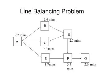
Readiness Assessment Test (RAT) Draw the precedence diagram for the tasks shown below
F C B G J K A H D E I RAT – Solution Precedence Chart :
Optimal Solutions • Imagine a decision tree containing all possible sequences of tasks that obey the precedence constraints. • “0” node is called root of the tree, terminal nodes at the other end are called the leaves. • A unique path leads from root to each leaf. • Each leaf represents a complete sequence. • Each feasible sequence is represented by exactly one leaf. • Best solution is found by examining every path.
Tree Generation • Backtracking – Allows both symmetric exploration of the tree and efficient storage of our location and history during exploration. • General applicability is to an environment in which N sequential decisions are to be made. • In generating the tree of possible sequences, the order of performing the assembly tasks is important rather than the workstations. • Tree initially grows by selecting first alternative at each stage until there is a complete assembly sequence
Tree Generation – Cont… • Backtrack until we reach the first node of the unexplored branch. • Continue moving forward, decision by decision, as far as possible. • Process continues until all possible leaves are explored. • A task is fittable if it satisfies three conditions. • Task must fit in the remaining idle time of the station. • It must be currently unassigned. • All its predecessors are assigned.
1. Setup k = 1, p = 0 ck = C, B = 0 4. Open New Station k = k+1 ck = C Yes 2. Select new task Find i’ = lowest i i fittable, i>B i > i* unless new station . i* > 0 ? No No No Yes i’ exist ? ck = C ? p = 0 ? No Yes Yes i* = i’ Stop Enumeration Complete 3. Assign task Ai* = k, p = p+1 ck = ck – ti* TAp = i*, B = 0 7. Backtrack to B. (Remove B from Station K) If ck = C, k = k-1 B = Tap, AB = 0 ck = ck+tB p = p-1, i* = 0 6. Sequence complete Save if best solution No Yes p = N ? Tree Generation Algorithm 0. Input Bound and task data
Tree Exploration • Creating only those new nodes required to find or disprove the existence of a better solution. • In practice, we need not create each node of the tree. • At any partial sequence node, if we can establish that all completions of this partial sequence are non-optimal; then we will start backtracking immediately instead of completing a sequence. • Two Rules – Problem Structure Rules & Fathoming Rules.
Problem Structure Rules • Basic Optimality Principle – Never close a workstation while “fittable” tasks remain. • Open a new workstation once when necessitated by time. • Long task becomes a station only when no other task can feasibly fit in the same station. • A lower bound on the number of workstations needed is useful in determining if we have an optimal solution.
Fathoming Rules • These rules help us to prune the tree rapidly. • Allows us to implicitly consider all leaves without explicitly enumerating many of them. • Rules only be checked when a new workstation must be opened. Rule 1 : Task Dominance • Suppose Task i can be feasibly replaced by a longer task j and all successors must also follow j. • If we substitute, we reduce the workload without losing any possible sequence completions.
Fathoming Rules – Cont… Rule 2 : Station Dominance • Suppose we try to form a station that is identical to a “first” station that was explored earlier. • As no new sequences can be considered, new node is fathomed. Rule 3 : Solution Dominance • We know that K0 gives a lower bound on optimal number of solutions. • We can stop once we have got a solution as that of lower bound
Fathoming Rules – Cont… Rule 4 : Bound Violation • Suppose we have K workstations. This is optimal unless a K – 1 solution is found. • Let Ai be the station to which task iis assigned. If we require at most K – 1 stations, the upper bound is given by • Nodes containing at least one of Ai outside these bounds can be pruned from the tree.
Fathoming Rules – Cont… Rule 5 : Excessive Idle Time • Whenever cumulative idle time exceeds (K – 1)C – i ti ,we may not fathom the partial sequence All the above mentioned fathoming rules are adapted from FABLE – Fast Algorithmfor Balancing LinesEffectivelydescribed by Johnson
Example Solution Product Structure Rules : • Task Time Augmentation Longest Station = tk = 46 Shortest Station = tc= 5 tk+ tc C. So task would require own station. • Solution Lower Bound Lower Bound K0 = 3 Only one task exceeds C/2 and two tasks exceeding C/3. No better solution exists now..
Example Solution – Cont… Fathoming Rules : • Task Dominance Several Tasks can be replaced. Task Pairs satisfying the relationship are (j, d), (j, e), (j, f), (j, g), (j, h), (j, i), (i, f), (e, a), (e, h), (e, g), (e, d) • Task Bound Violation Assume current best solution has four stations. The natural ordering being (a, b, c, d, e), (f, g, h), (i, j, k), (l) Still need to search for three-station solution. Bound violations will be useful.
f g h 7 8 9 e j 5 6 g h i d 10 11 12 4 c e f 3 h i j k l 14 15 16 17 18 19 20 g b 2 13 a 1 Example Solution – Tree Generation 0
Team Exercise Consider the five assembly tasks given below Evaluate each sequence in the tree to determine the number of workstation required. List all optimal sequences
Exercise Solution Workstation Optimal b c d e 4 Yes 0 a c b d e 4 Yes d b e 4 Yes e b 4 Yes
Practical Issues • C has been fixed so far but in reality we only forecast demand. • C should be set such that i ti / C is an integer or jus less than an integer. • Randomness in performance times exists. • Let i2 Variance of performance times. ij Correlation between tasks i and j. sk Random variable for the time required by station k for a cycle Sk Set of tasks assigned to station k.
Practical Issues – Cont… From basic statistics we know When added to the station, the task must satisfy
Operation Time Predecessors a 3 - b 5 - c 10 a, b d 11 c e 24 c f 26 d g 24 e h 15 g Assignment Solve by implicit enumeration technique and find the optimal solution