Introduction to Linear Programming
Introduction to Linear Programming. A Linear Programming model seeks to maximize or minimize a linear function, subject to a set of linear constraints. The linear model consists of the following components: A set of decision variables. An objective function. A set of constraints.

Introduction to Linear Programming
E N D
Presentation Transcript
Introduction to Linear Programming • A Linear Programming model seeks to maximize or minimize a linear function, subject to a set of linear constraints. • The linear model consists of the followingcomponents: • A set of decision variables. • An objective function. • A set of constraints.
Introduction to Linear Programming • The Importance of Linear Programming • Many real world problems lend themselves to linear programming modeling. • Many real world problems can be approximated by linear models. • There are well-known successful applications in: • Manufacturing • Marketing • Finance (investment) • Advertising • Agriculture
Introduction to Linear Programming • The Importance of Linear Programming • There are efficient solution techniques that solve linear programming models. • The output generated from linear programming packages provides useful “what if” analysis.
Introduction to Linear Programming • Assumptions of the linear programming model • The parameter values are known with certainty. • The objective function and constraints exhibit constant returns to scale. • There are no interactions between the decision variables (the additivity assumption). • The Continuity assumption: Variables can take on any value within a given feasible range.
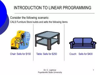
The Galaxy Industries Production Problem – A Prototype Example • Galaxy manufactures two toy doll models: • Space Ray. • Zapper. • Resources are limited to • 1000 pounds of special plastic. • 40 hours of production time per week.
The Galaxy Industries Production Problem – A Prototype Example • Marketing requirement • Total production cannot exceed 700 dozens. • Number of dozens of Space Rays cannot exceed number of dozens of Zappers by more than 350. • Technological input • Space Rays requires 2 pounds of plastic and • 3 minutes of labor per dozen. • Zappers requires 1 pound of plastic and • 4 minutes of labor per dozen.
8(450) + 5(100) The Galaxy Industries Production Problem – A Prototype Example • The current production plan calls for: • Producing as much as possible of the more profitable product, Space Ray ($8 profit per dozen). • Use resources left over to produce Zappers ($5 profit per dozen), while remaining within the marketing guidelines. • The current production plan consists of: • Space Rays = 450 dozen • Zapper = 100 dozen • Profit = $4100 per week
Management is seeking a production schedule that will increase the company’s profit.
A linear programming model can provide an insight and an intelligent solution to this problem.
The Galaxy Linear Programming Model • Decisions variables: • X1 = Weekly production level of Space Rays (in dozens) • X2 = Weekly production level of Zappers (in dozens). • Objective Function: • Weekly profit, to be maximized
The Galaxy Linear Programming Model Max 8X1 + 5X2 (Weekly profit) subject to 2X1 + 1X2£ 1000 (Plastic) 3X1 + 4X2£ 2400 (Production Time) X1 + X2£ 700 (Total production) X1 - X2£ 350 (Mix) Xj> = 0, j = 1,2 (Nonnegativity)