Download
1 / 58
650 likes | 812 Views
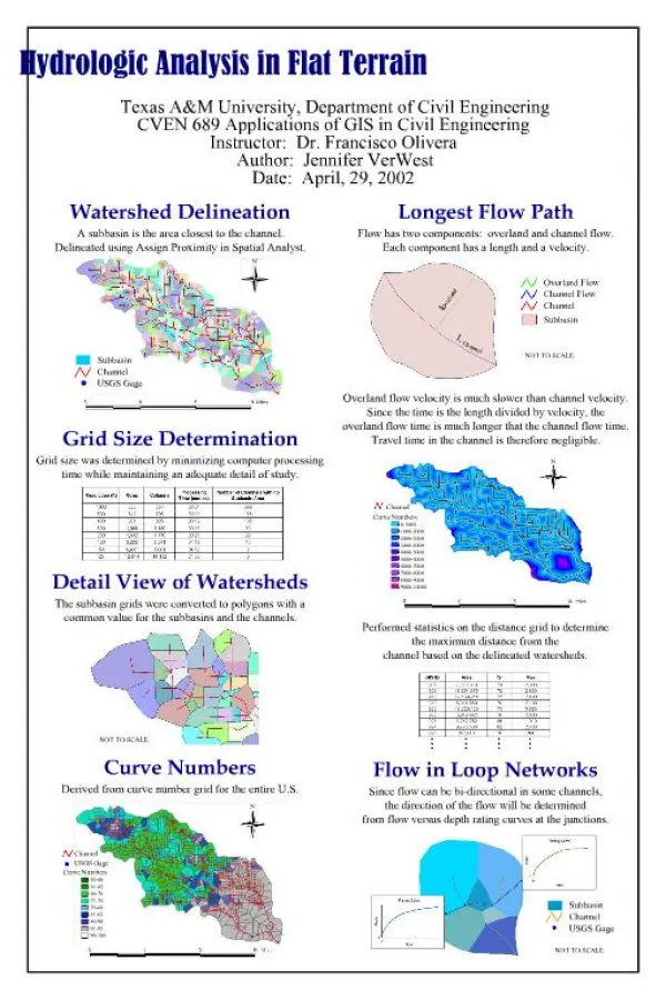
Explore grid-based terrain flow data modeling, stream threshold delineation, drainage density, flow direction models, and terrain stability mapping in ArcGIS for efficient hydrologic analysis.

E N D
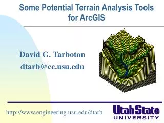
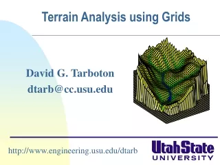
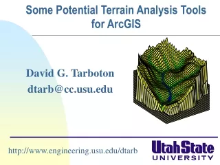
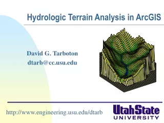
Hydrologic Terrain Analysis in ArcGIS David G. Tarboton dtarb@cc.usu.edu http://www.engineering.usu.edu/dtarb
Outline • Grid based terrain flow data model • Objective stream threshold delineation • Variable drainage density • D multiple flow direction model • Flow algebra • Terrain stability mapping (SINMAP)
Terrain Data Models Grid TIN Contour and flowline
Duality between Terrain and Drainage Network • Flowing water erodes landscape and carries away sediment sculpting the topography • Topography defines drainage direction on the landscape and resultant runoff and streamflow accumulation processes
Grid based terrain flow data model A grid defines geographic space as a matrix of identically-sized square cells. Each cell holds a numeric value that measures a geographic attribute (like elevation) for that unit of space.
30 67 56 49 4 3 2 5 1 52 48 37 6 7 8 58 55 22 Eight Direction Pour Point Model D8 Slope = Drop/Distance Steepest down slope direction
Grid based terrain flow data model Grid network Eight direction pour point model D8 4 3 2 1 1 1 1 1 5 6 7 1 1 4 3 3 1 8 1 2 1 1 12 Drainage Area 1 1 1 2 16 2 1 3 6 25
Flow Accumulation Grid. Area draining in to a grid cell 0 0 0 0 0 0 0 0 0 0 0 3 2 2 0 3 2 0 0 2 0 1 0 0 11 0 0 1 0 11 0 0 0 1 15 0 0 1 0 15 1 0 2 5 24 2 5 0 1 24 ArcHydro Page 72
0 0 0 0 0 3 2 0 0 2 0 0 1 0 11 0 0 1 0 15 2 5 0 1 24 Channel or Stream Raster Flow Accumulation > 5 Cell Threshold
1 1 2 1 2 3 5 3 3 5 4 4 4 4 4 6 6 6 Stream Segments in a Grid Cell Network 5 5
Stream links grid for the San Marcos subbasin 201 172 202 203 206 204 Each link has a unique identifying number 209 ArcHydro Page 74
Catchments • For every stream segment, there is a corresponding catchment • Catchments are a tessellation of the landscape through a set of physical rules
Delineation of Channel Networks and Catchments 500 cell theshold 1000 cell theshold
AREA 2 3 AREA 1 12 How to decide on stream delineation threshold ? Why is it important?
Hydrologic processes are different on hillslopes and in channels. It is important to recognize this and account for this in models. Drainage area can be concentrated or dispersed (specific catchment area) representing concentrated or dispersed flow. Objective determination of channel network drainage density
“landscape dissection into distinct valleys is limited by a threshold of channelization that sets a finite scale to the landscape.” (Montgomery and Dietrich, 1992, Science, vol. 255 p. 826.) One contributing area threshold does not fit all watersheds. Map stream networks from the DEM at the finest resolution consistent with observed stream network geomorphology ‘laws’.
Strahler Stream Order Order 5 Order 1 • most upstream is order 1 • when two streams of a order i join, a stream of order i+1 is created • when a stream of order i joins a stream of order i+1, stream order is unaltered Order 3 Order 4 Order 2
Constant Stream Drops Law Broscoe, A. J., (1959), "Quantitative analysis of longitudinal stream profiles of small watersheds," Office of Naval Research, Project NR 389-042, Technical Report No. 18, Department of Geology, Columbia University, New York.
Nodes Links Single Stream Note that a “Strahler stream” comprises a sequence of links (reaches or segments) of the same order Stream DropElevation difference between ends of stream
Look for statistically significant break in constant stream drop property Break in slope versus contributing area relationship Physical basis in the form instability theory of Smith and Bretherton (1972), see Tarboton et al. 1992 Suggestion: Map channel networks from the DEM at the finest resolution consistent with observed channel network geomorphology ‘laws’.
T-Test for Difference in Mean Values 72 130 0 T-test checks whether difference in means is large (> 2) when compared to the spread of the data around the mean values
200 grid cell constant drainage area based stream delineation
100 grid cell constant drainage area threshold stream delineation
Local Curvature Computation(Peuker and Douglas, 1975, Comput. Graphics Image Proc. 4:375) 43 48 48 51 51 56 41 47 47 54 54 58
Curvature based stream delineation with threshold by constant drop analysis
Channel network delineation, other options 4 3 2 1 1 1 1 1 1 1 1 1 1 5 6 7 1 1 1 4 2 3 2 2 3 1 1 Grid Order 8 1 1 1 2 1 1 1 1 3 12 1 1 1 1 1 1 2 1 16 3 1 2 1 1 2 3 6 2 25 3 Contributing Area
? Limitation due to 8 grid directions. Flow Direction Field — if the elevation surface is differentiable (except perhaps for countable discontinuities) the horizontal component of the surface normal defines a flow direction field.
D Multiple flow direction model Proportion flowing to neighboring grid cell 2 is 1/(1 + 2) Proportion flowing to neighboring grid cell 1 is 2/(1 + 2) Tarboton, D. G., (1997), "A New Method for the Determination of Flow Directions and Contributing Areas in Grid Digital Elevation Models," Water Resources Research, 33(2): 309-319.) (http://www.engineering.usu.edu/cee/faculty/dtarb/dinf.pdf)
Contributing Area using D Contributing Area using D8
Useful for example to track where sediment or contaminant moves
Useful for example to track where a contaminant may come from
Useful for a tracking contaminant or compound subject to decay or attenuation
Useful for a tracking a contaminant released or partitioned to flow at a fixed threshold concentration
Transport limited accumulation Useful for modeling erosion and sediment delivery, the spatial dependence of sediment delivery ratio and contaminant that adheres to sediment
Terrain Stability Mapping With Bob Pack. http://www.engineering.usu.edu/dtarb/sinmap.htm
D h SINMAP Theoretical Basis Infinite Plane Slope Stability Model Dw D FS=Factor of Safety R = DEM source q = slope where Relative Wetness Density Ratio Dimensionless Cohesion
DEM Governs Slope & Flow Accumulation Digital Terrain Model (DTM) DTM Quality Flow Accumulation (a) Slope (θ)
Probabilistic Formulation Shear Strength P(FS>1) Slope Flow Accumulation Wetness MODEL SI=FS & Soil/Root Cohesion
Interactive Calibration Selection of ranges of Φ, R/T & c moves position of stability class breaks Selection of range of R/T moves position of wetness class breaks
Example Result – Foster Ck DRAINAGE AREA UPSLOPE UNSTABLE STABLE SATURATED UNSATURATED Class 1 2 3 4 5 6 SLOPE