Dynamic Behavior of Closed-Loop Control Systems
480 likes | 1k Views
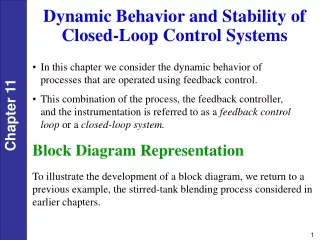
Dynamic Behavior of Closed-Loop Control Systems. Chapter 11. Chapter 11.

Dynamic Behavior of Closed-Loop Control Systems
E N D
Presentation Transcript
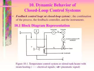
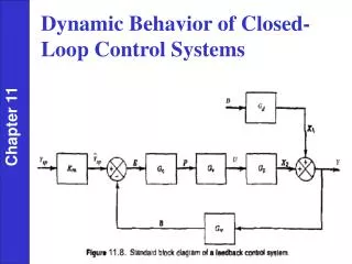
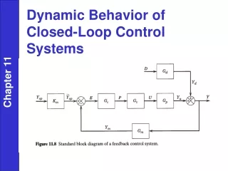
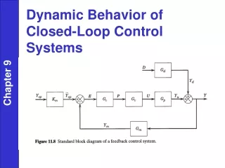
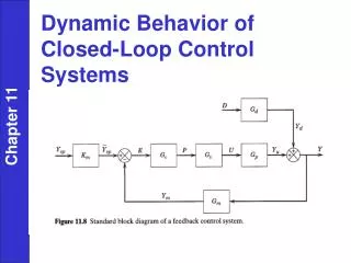
Next, we develop a transfer function for each of the five elements in the feedback control loop. For the sake of simplicity, flow rate w1 is assumed to be constant, and the system is initially operating at the nominal steady rate. Process In section 4.1 the approximate dynamic model of a stirred-tank blending system was developed: Chapter 11 where
The symbol denotes the internal set-point composition expressed as an equivalent electrical current signal. is related to the actual composition set point by the composition sensor-transmitter gain Km: Chapter 11
Current-to-Pressure (I/P) Transducer The transducer transfer function merely consists of a steady-state gain KIP: Chapter 11 Control Valve As discussed in Section 9.2, control valves are usually designed so that the flow rate through the valve is a nearly linear function of the signal to the valve actuator. Therefore, a first-order transfer function is an adequate model
Composition Sensor-Transmitter (Analyzer) We assume that the dynamic behavior of the composition sensor-transmitter can be approximated by a first-order transfer function, but τm is small so it can be neglected. Controller Suppose that an electronic proportional plus integral controller is used. Chapter 11 where and E(s) are the Laplace transforms of the controller output and the error signal e(t). Kc is dimensionless.
1. Summer 2. Comparator Chapter 11 3. Block • Blocks in Series are equivalent to...
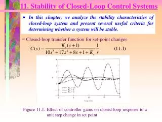
“Closed-Loop” Transfer Functions • Indicate dynamic behavior of the controlled process • (i.e., process plus controller, transmitter, valve etc.) • Set-point Changes (“Servo Problem”) Assume Ysp 0 and D = 0 (set-point change while disturbance change is zero) Chapter 11 (11-26) • Disturbance Changes (“Regulator Problem”) Assume D 0 and Ysp = 0 (constant set-point) (11-29) *Note same denominator for Y/D, Y/Ysp.
Chapter 11 Figure 11.16 Block diagram for level control system.
EXAMPLE 1: P.I. control of liquid level Block Diagram: Chapter 11
Assumptions 1. q1, varies with time; q2 is constant. 2. Constant density and x-sectional area of tank, A. 3. (for uncontrolled process) 4. The transmitter and control valve have negligible dynamics (compared with dynamics of tank). 5. Ideal PI controller is used (direct-acting). Chapter 11 For these assumptions, the transfer functions are:
The closed-loop transfer function is: (11-68) Substitute, (2) Chapter 11 Simplify, (3) Characteristic Equation: (4) Recall the standard 2nd Order Transfer Function: (5)
To place Eqn. (4) in the same form as the denominator of the T.F. in Eqn. (5), divide by Kc, KV, KM : Comparing coefficients (5) and (6) gives: Chapter 11 Substitute, For 0 < < 1 , closed-loop response is oscillatory. Thus decreased degree of oscillation by increasing Kc or I (for constant Kv, KM, and A). • unusual property of PI control of integrating system • better to use P only
Stability of Closed-Loop Control Systems Chapter 11
Proportional Control of First-Order Process Set-point change: Chapter 11
Set-point change = M Chapter 11 Offset = See Section 11.3 for tank example
Closed-Loop Transfer function approach: Chapter 11 First-order behavior closed-loop time constant (faster, depends on Kc)
General Stability Criterion Most industrial processes are stable without feedback control. Thus, they are said to be open-loop stable or self-regulating. An open-loop stable process will return to the original steady state after a transient disturbance (one that is not sustained) occurs. By contrast there are a few processes, such as exothermic chemical reactors, that can be open-loop unstable. Definition of Stability. An unconstrained linear system is said to be stable if the output response is bounded for all bounded inputs. Otherwise it is said to be unstable. Chapter 11
is unspecified Effect of PID Control on a Disturbance Change For a regulator (disturbance change), we want the disturbance effects to attenuate when control is applied. Consider the closed-loop transfer function for proportional control of a third-order system (disturbance change). Chapter 11 Kc is the controller function, i.e., .
Let If Kc = 1, Chapter 11 Since all of the factors are positive, , the step response will be the sum of negative exponentials, but will exhibit oscillation. If Kc = 8, Corresponds to sine wave (undamped), so this case is marginally stable.
If Kc = 27 Since the sign of the real part of the root is negative, we obtain a positive exponential for the response. Inverse transformation shows how the controller gain affects the roots of the system. Chapter 11 Offset with proportional control (disturbance step-response; D(s) =1/s )
Therefore, if Kc is made very large, y(t) approaches 0, but does not equal zero. There is some offset with proportional control, and it can be rather large when large values of Kc create instability. Integral Control: Chapter 11 For a unit step load-change and Kc=1, no offset (note 4th order polynomial)
Analysis of roots of characteristic equation is one way to analyze controller behavior PI Control: no offset adjust Kc and I to obtain satisfactory response (roots of equation which is 4th order). Chapter 11 PID Control:(pure PID) No offset, adjust Kc, I , D to obtain satisfactory result (requires solving for roots of 4th order characteristic equation).
Rule of Thumb: Closed-loop response becomes less oscillatory and more stable by decreasing Kc or increasing tI. General Stability Criterion Consider the “characteristic equation,” Note that the left-hand side is merely the denominator of the closed-loop transfer function. Chapter 11 The roots (poles) of the characteristic equation (s - pi) determine the type of response that occurs: Complex roots oscillatory response All real roots no oscillations ***All roots in left half of complex plane = stable system
Chapter 11 Figure 11.25 Stability regions in the complex plane for roots of the characteristic equation.
Stability Considerations • Feedback control can result in oscillatory or even unstable closed-loop responses. Chapter 11 • Typical behavior (for different values of controller gain, Kc).
Roots of 1 + GcGvGpGm Chapter 11 (Each test is for different value of Kc) (Note complex roots always occur in pairs) Figure 11.26 Contributions of characteristic equation roots to closed-loop response.
Routh Stability Criterion Characteristic equation Chapter 11 (11-93) Where an >0 . According to the Routh criterion, if any of the coefficients a0, a1, …, an-1 are negative or zero, then at least one root of the characteristic equation lies in the RHP, and thus the system is unstable. On the other hand, if all of the coefficients are positive, then one must construct the Routh Array shown below:
Chapter 11 For stability, all elements in the first column must be positive.
The first two rows of the Routh Array are comprised of the coefficients in the characteristic equation. The elements in the remaining rows are calculated from coefficients by using the formulas: (11-94) Chapter 11 (11-95) . . (11-96) (11-97) (n+1 rows must be constructed; n = order of the characteristic eqn.)
Application of the Routh Array: Characteristic Eqn is We want to know what value of Kc causes instability, I.e., at least one root of the above equation is positive. Using the Routh array, Chapter 11 Conditions for Stability The important constraint is Kc<8. Any Kc8 will cause instability.
Figure 11.29 Flowchart for performing a stability analysis. Chapter 11
Additional Stability Criteria • 1. Bode Stability Criterion • Ch. 14 - can handle time delays • 2. Nyquist Stability Criterion • Ch. 14 Chapter 11
Direct Substitution Method Imaginary axis is the dividing line between stable and unstable systems. • Substitute s = jw into characteristic equation • Solve for Kcm and wc • (a) one equation for real part • (b) one equation for imaginary part • Example (cf. Example 11.11) • characteristic equation: 1 + 5s + 2Kce-s = 0 (11-101) • set s = jw 1 + 5jw + 2Kce-jw = 0 • 1 + 5jw + 2Kc (cos(w) – j sin(w)) = 0 Chapter 11
Direct Substitution Method (continued) Re: 1 + 2Kccos w = 0 (1) Im: 5w – 2Kc sin w = 0 (2) solve for Kcin (1) and substitute into (2): Chapter 11 Solve for w: wc = 1.69 rad/min (96.87°/min) from (1) Kcm = 4.25 (vs. 5.5 using Pade approximation in Example 11.11)
Chapter 11 Previous chapter Next chapter