Download

1 / 56
570 likes | 910 Views
An Epidemiological Approach to Diagnostic Process. Steve Doucette, BSc, MSc Email: sdoucette@ohri.ca Ottawa Health Research Institute Clinical Epidemiology Program The Ottawa Hospital (General Campus).

E N D
An Epidemiological Approach to Diagnostic Process Steve Doucette, BSc, MSc Email: sdoucette@ohri.ca Ottawa Health Research Institute Clinical Epidemiology Program The Ottawa Hospital (General Campus)
Topics to be covered…-Through use of illustrative examples involving clinical trials, we’ll discuss the following: • Diagnostic and Screening tests • Conditional Probability • The 2 X 2 Table • Sensitivity, Specificity, Predictive Value • ROC curves • Bayes Theorem • Likelihood and Odds
What are Diagnostic & Screening tests? • Important part of medical decision making • In practice, many tests are used to obtain diagnoses • Screening tests: Are used for persons who are asymptomatic but who may have early disease or disease precursors • Diagnostic tests: Are used for persons who have a specific indication of possible illness
Screening - the proportion of affected persons is likely to be small (Breast Cancer) Early detection of disease is helpful only if early intervention is helpful Diagnostic tests - many patients have medical problems that require investigation Usually to diagnosis disease for immediate treatment What’s the difference?
Why conduct diagnostic tests? • Does a positive acid-fast smear guarantee that the patient has active tuberculosis? NO • Does a toxic digoxin concentration inevitably signify digitalis intoxication? NO • By having a factor VIII ratio < 0.8, are you automatically known to be a hemophilia carrier? NO
Not all tests are perfect…but • A positive test results should increase the “probability” that the disease is present. • “Good” tests aim to be: -sensitive -specific -predictive -accurate
Terminology • Sensitive test: If all persons with the disease have “positive” tests, we say the test is sensitive to the presence of disease • Specific test: If all persons without the disease test “negative”, we say the rest is specific to the absence of the disease • Predictive (positive & negative) test: If the results of the test are indicative of the true outcome
Terminology • Accuracy: The accuracy of a test expresses includes all the times that this test resulted in a correct result. It represents true positive and negative results among all the results of the test. • Prevalence: The number or proportion of cases of a given disease or other attribute that exists in a defined population at a specific time.
Terminology • Probability: A number expressing the likelihood that a specific event will occur, expressed as the ratio of the number of actual occurrences to the number of possible occurrences. P(A) = a / n
Terminology • Conditional Probability: A number expressing the likelihood that a specific event will occur, GIVEN that certain conditions hold. • Sensitivity, Specificity, Positive & Negative Predictive Values are all conditional probabilities. P(A|B)
Terminology • Sensitivity: The proportion of positive results among all the patients that have certain disease. • Specificity: The proportion of negative results among all the patients that did not have disease. • Positive Predictive Value: The proportion of patients who have disease among all the patients that tested positive. • Negative Predictive Value: The proportion of patients who do not have disease among all the patients that tested negative. These are all conditional probabilities!!
+ Test Result - The 2 X 2 Table Truth - + A B A+B C D C+D B+D A+B+C+D A+C
The 2 X 2 Table Formulas: Truth + - Sensitivity = a / a+c A B + Test Result Specificity = d / b+d - C D Accuracy = a+d / a+b+c+d Prevalence = a+c / a+b+c+d Predictive Value: Positive Test = a+b / a+b+c+d positive = a / a+b Negative Test = c+d / a+b+c+d negative = d / c+d Diseased = a+c / a+b+c+d Not Diseased = b+d / a+b+c+d
The 2 X 2 Table • Example: Testing for Genetic Hemophilia -A method for testing whether an individual is a carrier of hemophilia (a bleeding disorder) takes the ratio of factor VIII activity to factor VIII antigen. This ratio tends to be lower in carriers thus providing a basis for diagnostic testing. In this example, a ratio < 0.8 gives a positive test result. Results: -38 tested positive, 6 incorrectly. -28 tested negative, 2 incorrectly.
The 2 X 2 Table Carrier State Carrier Non-Carrier + 32 38 6 F8 < 0.8 Test Result - 30 2 28 F8 > 0.8 68 34 34
The 2 X 2 Table Carrier State Exercise: Non-Carrier Carrier 6 32 38 + Sensitivity = Test Result Specificity = 28 2 - 30 Accuracy = 68 34 34 Prevalence = Predictive Value: Positive Test = positive = Negative Test = negative = Diseased = Not Diseased =
The 2 X 2 Table • Example: Testing for digoxin toxicity -A method for testing whether an individual is a digoxin toxic measures serum digoxin levels. A cut off value for serum concentration provides a basis for diagnostic testing. Results: -39 tested positive, 14 incorrectly. -96 tested negative, 18 incorrectly.
The 2 X 2 Table Toxicity D+ D- T+ 25 39 14 Test Result T- 96 18 78 135 43 92
The 2 X 2 Table Toxicity Exercise: D- D+ 25 14 39 T+ Sensitivity = Test Result Specificity = 78 18 T- 96 Accuracy = 135 43 92 Prevalence = Predictive Value: Positive Test = positive = Negative Test = negative = Diseased = Not Diseased =
Sensitivity & Specificity – Trade off • Ideally we would like to have 100% sensitivity and specificity. • If we want our test to be more sensitive, we will pay the price of losing specificity. • Increasing specificity will result in a decrease in sensitivity.
Back to Hemophilia example… Non Carrier Non Carrier Carrier Carrier 32 6 13 33 38 46 + + Test Result Test Result 28 2 1 21 - - 30 22 68 68 34 34 34 34 Exercise: Exercise: Sensitivity = 33/(33+1) = 0.97 Sensitivity = 32/(32+2) = 0.94 Specificity = 21/(21+13) = 0.62 Specificity = 28/(28+6) = 0.82 Predictive Value: Predictive Value: positive = 33/(33+13) = 0.72 positive = 32/(32+6) = 0.84 negative = 21/(21+1) = 0.95 negative = 28/(28+2) = 0.93
Example 2: How can prevalence affect predictive value? Non Carrier Non Carrier Carrier Carrier 32 6 600 32 38 632 + + Test Result Test Result 28 2 2 2800 - - 30 2802 68 3034 34 34 34 3400 Exercise: Exercise: Sensitivity = 32/(32+2) = 0.94 Sensitivity = 32/(32+2) = 0.94 Specificity = 2800/(2800+600) = 0.82 Specificity = 28/(28+6) = 0.82 Predictive Value: Predictive Value: positive = 32/(32+600) = 0.05 positive = 32/(32+6) = 0.84 negative = 2800/(2800+2)= 0.999 negative = 28/(28+2) = 0.93
Summary • The 2 X 2 Table allows us to compute sensitivity, specificity, and predictive values of a test. • The prevalence of a disease can affect how our test results should be interpreted.
ROC Curves - Introduction Cut-off value for test TP=a FP=b FN=c With Disease TN=d Without Disease TP TN FN FP 0.5 0.6 0.7 0.8 0.9 1.0 1.1 POSITIVE NEGATIVE Test Result
ROC Curves - Introduction Cut-off value for test With Disease Without Disease TP TN FP FN 0.5 0.6 0.7 0.8 0.9 1.0 1.1 POSITIVE NEGATIVE Test Result
ROC Curves • An ROC curve is a graphical representation of the trade off between the false negative and false positive rates for every possible cut off. Equivalently, the ROC curve is the representation of the tradeoffs between sensitivity (Sn) and specificity (Sp). • By tradition, the plot shows 1-Sp on the X axis and Sn on the Y axis.
ROC Curves • Example: Given 5 different cut offs for the hemophilia example: 0.5, 0.6, 0.7, 0.8, 0.9. What might an ROC curve look like?
ROC Curves 1 0.8 0.6 0.4 Sensitivity 0.2 0 0 0.2 0.4 0.6 0.8 1 1- Specificity
1 0.8 0.6 0.4 Sensitivity 0.2 0 0 0.2 0.4 0.6 0.8 1 1- Specificity ROC Curves • We are usually happy when the ROC curve climbs rapidly towards upper left hand corner of the graph. This means that Sensitivity and specificity is high. We are less happy when the ROC curve follows a diagonal path from the lower left hand corner to the upper right hand corner. This means that every improvement in false positive rate is matched by a corresponding decline in the false negative rate
1 0.8 0.6 0.4 Sensitivity 0.2 0 0 0.2 0.4 0.6 0.8 1 1- Specificity ROC Curves • Area under ROC curve: 1 = Perfect diagnostic test 0.5 = Useless diagnostic test • If the area is 1.0, you have an ideal test, because it achieves both 100% sensitivity and 100% specificity. • If the area is 0.5, then you have a test which has effectively 50% sensitivity and 50% specificity. This is a test that is no better than flipping a coin.
What's a good value for the area under the curve? • Deciding what a good value is for area under the curve is tricky and it depends a lot on the context of your individual problem. • What are the cost associated with misclassifying someone as non-diseased when in fact they were? (False Negative) • What are the costs associated with misclassifying someone as diseased when in fact they weren’t? (False Positive)
ROC Curves 1 0.8 0.6 0.4 Test 1 Sensitivity Test 2 0.2 Test 3 0 0 0.2 0.4 0.6 0.8 1 1- Specificity
P(B|A) P(A) P(A|B) = P(B|A) P(A) + P(B|not A) P(not A) Note: P(B) = 0 Bayes Theorem • The 2 x 2 table offers a direct way to compute the positive and negative predictive values. • Bayes Theorem gives identical results without constructing the 2 x 2 table.
P(T+|D+) P(D+) P(T-|D-) P(D-) P(D+|T+) = P(D-|T-) = P(T+|D+) P(D+) + P(T+|D-) P(D-) P(T-|D-) P(D-) + P(T-|D+) P(D+) Bayes Theorem • Applying these results: Positive predictive Value = P(D+|T+) Sensitivity 1- Specificity Specificity Negative predictive Value = P(D-|T-) 1- Sensitivity
How does Bayes Rule help? • Example: Investigators have developed a diagnostic test, and in a population we know the tests’ sensitivity and specificity. • The results of a diagnostic test will allow us to compute the probability of disease. • The new, updated, probability from new information is called the posterior probability.
Back to Digoxin example… • Say we know that someone’s probability of toxicity is 0.6. We now give them the diagnostic test and find out that their digoxin levels were high and they tested positive. What is the new probability of disease, given the positive test result information? P(T+|D+) P(D+) P(D+|T+) = P(T+|D+) P(D+) + P(T+|D-) P(D-)
P(T+|D+) P(D+) P(D+|T+) = P(T+|D+) P(D+) + P(T+|D-) P(D-) Back to Digoxin example… We know P(D+) = 0.6 From before, 1- 0. 6 = 0.4 Sensitivity = 25/(25+18) = 0.58 1- 0.85 = 0.15 Specificity = 78/(78+14) = 0.85 0.58*0.6 P(D+|T+) = = 0.85 0.58*0.6 + 0.15*0.4
P(T-|D-) P(D-) P(D-|T-) = P(T-|D-) P(D-) + P(T-|D+) P(D+) Back to Digoxin example… We know P(D+) = 0.6 1- 0.6 = 0.4 From before, Sensitivity = 25/(25+18) = 0.58 1- 0.58 = 0.42 Specificity = 78/(78+14) = 0.85 0.85*0.4 P(D-|T-) = = 0.57 0.85*0.4 + 0.42*0.6
Digoxin example continued… • What happens to the positive and negative predictive values if our ‘prior’ probability of disease, P(D+), changes… • Example 2: What is the new probability of disease given the same positive test, however the probability of disease was known to be 0.3 before testing?
P(T+|D+) P(D+) P(D+|T+) = P(T+|D+) P(D+) + P(T+|D-) P(D-) Back to Digoxin example… We know P(D+) = 0.3 From before, 1- 0. 3 = 0.7 Sensitivity = 25/(25+18) = 0.58 1- 0.85 = 0.15 Specificity = 78/(78+14) = 0.85 0.58*0.3 P(D+|T+) = = 0.62 0.58*0.3 + 0.15*0.7
P(T-|D-) P(D-) P(D-|T-) = P(T-|D-) P(D-) + P(T-|D+) P(D+) Back to Digoxin example… We know P(D+) = 0.3 1- 0.3 = 0.7 From before, Sensitivity = 25/(25+18) = 0.58 1- 0.58 = 0.42 Specificity = 78/(78+14) = 0.85 0.85*0.7 P(D-|T-) = = 0.83 0.85*0.7 + 0.42*0.3
Hemophilia example continued… Example: Mrs X. had positive lab results, what is the probability she was a carrier?? P(D+|T+) • Hemophilia is a genetic disorder. If Mrs. X mother was a carrier, Mrs. X would have a 50-50 chance of being a carrier. (Prior probability) • If all we knew was that her grandmother was a carrier, Mrs. X would have a 25% chance of being a carrier.
P(T+|D+) P(D+) P(D+|T+) = P(T+|D+) P(D+) + P(T+|D-) P(D-) Hemophilia example continued… From before, Sensitivity = 32/(32+2) = 0.94 Specificity = 28/(28+6) = 0.82 Grandmother was a carrier Mother was a carrier 0.94*0.25 0.94*0.5 = 0.64 = 0.84 P(D+|T+) = P(D+|T+) = 0.94*0.25 + 0.18*0.75 0.94*0.5 + 0.18*0.5
Summary • Bayes theorem allows us to calculate the positive and negative predictive values using only sensitivity, specificity, and the probability of disease (prevalence).
LR+ = Sensitivity LR- = 1-Sensitivity 1- Specificity Specificity Likelihood and Odds • Likelihood Ratio: • What would a good LR+ look like? HIGH LR+ and LOW LR- imply both sensitivity and specificity are close to 1
P(A) 2/3 P(A) 1- 2/3 1- P(A) P(NOT A) Likelihood and Odds • The odds in favor of ‘A’ is defined as: Odds in favor of A = = • Example: if P(A) = 2/3 then the odds in favor of A is: (or 2 to 1) = 2
2 odds 1 + 2 1 + odds Likelihood and Odds • We can also calculate probability knowing the odds of disease P(A) = • Example: if the odds = 2 (that is 2:1) then the probability in favor of A is: = 2/3
Likelihood and Odds • Some more simple examples: -The Odds in favor of heads when a coin is tossed is 1. (Ratio of 1:1) -The Odds in favor of rolling a ‘6’ on any throw of a fair die is 0.2. (Ratio of 1:5) -The Odds AGAINST rolling a ‘6’ on any throw of a fair die is 5. (Ratio of 5:1) -The Odds in favor of drawing an ace from an ordinary deck of playing cards is 1/12. (Ratio of 1:12)
Likelihood and odds • Recall, ‘prior’ probability was the known probability of outcome (ex. Disease) before our diagnostic test. • Posterior probability is the probability of outcome (ex. Disease) after updating results from our diagnostic test. • Prior and posterior odds have the same definition.
Posterior Odds Posterior odds in favor of A Prior odds in favor of A Likelihood ratio X = LR+ if they tested positive LR- if they tested negative