Download
1 / 40
410 likes | 695 Views
Regularization and Feature Selection in Least-Squares Temporal Difference Learning. J. Zico Kolter and Andrew Y. Ng Computer Science Department Stanford University June 16 th , ICML 2009. TexPoint fonts used in EMF.

E N D
Regularization and Feature Selection in Least-Squares Temporal Difference Learning J. Zico Kolter and Andrew Y. NgComputer Science DepartmentStanford University June 16th, ICML 2009 TexPoint fonts used in EMF. Read the TexPoint manual before you delete this box.: AAAAAAAAAAAAAAA
Outline • RL with (linear) function approximation • Least-squares temporal difference (LSTD) algorithms very effective in practice • But, when number of features is large, can be expensive and over-fit to training data
Outline • RL with (linear) function approximation • Least-squares temporal difference (LSTD) algorithms very effective in practice • But, when number of features is large, can be expensive and over-fit to training data • This work: present method for feature selection in LSTD (via L1 regularization) • Introduce notion of L1-regularized TD fixed points, and develop an efficient algorithm
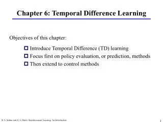
Problem Setup • Markov chain M = (S, R, P, ) • Set of states S • Reward function R(s) • Transition Probabilities P(s’|s) • Discount factor • Want to compute the value function for the Markov chain
Problem Setup • Markov chain M = (S, R, P, ) • Set of states S • Reward function R(s) • Transition Probabilities P(s’|s) • Discount factor • Want to compute the value function for the Markov chain • But, problem is hard because: • Don’t know the true state transitions / reward (only have access to samples) • State space is too large to represent the value function explicitly
TD Algorithms • Temporal difference (TD) family of algorithms (Sutton, 1988) addresses this problem setting • In particular, focus on Least-Squares Temporal Difference (LSTD) algorithms (Bradtke and Barto, 1996; Boyan, 1999, Lagoudakis and Parr, 2003) • work well in practice, make efficient use of data
Brief LSTD Overview • Represent value function using linear approximation
Brief LSTD Overview • Represent value function using linear approximation parameter vector
Brief LSTD Overview • Represent value function using linear approximation state features
Brief LSTD Overview • TD methods seek parameters w that satisfy the following fixed-point equation
Brief LSTD Overview • TD methods seek parameters w that satisfy the following fixed-point equation optimization variable
Brief LSTD Overview • TD methods seek parameters w that satisfy the following fixed-point equation matrix of all state features
Brief LSTD Overview • TD methods seek parameters w that satisfy the following fixed-point equation vector of all rewards
Brief LSTD Overview • TD methods seek parameters w that satisfy the following fixed-point equation Matrix of transition probabilities
Brief LSTD Overview • TD methods seek parameters w that satisfy the following fixed-point equation • Also sometimes written (equivalently) as
Brief LSTD Overview • TD methods seek parameters w that satisfy the following fixed-point equation • Also sometimes written (equivalently) as LSTD finds a w that approximately satisfies this equation using only samples from the MDP (gives closed form expression for optimal w)
Problems with LSTD • Requires storing/inverting k x k matrix • Can be extremely slow for large k • In practice, often means that practitioner puts great effort into picking a few “good” features • For many features / few samples, LSTD can over-fit to training data
Regularized LSTD • Introduce regularization term into LSTD fixed point equation
Regularized LSTD • Introduce regularization term into LSTD fixed point equation • In particular, focus on L1 regularization • Encourages sparsity in feature weights (i.e., feature selection) • Avoids over-fitting to training samples • Avoids storing/inverting full k x k matrix
Regularized LSTD Solution • Unfortunately, for L1 regularized LSTD • No closed-form solution for optimal w • Optimal w cannot even be expressed as solution to convex optimization problem
Regularized LSTD Solution • Unfortunately, for L1 regularized LSTD • No closed-form solution for optimal w • Optimal w cannot even be expressed as solution to convex optimization problem • Fortunately, can be solved efficiently using algorithm similar to Least Angle Regression (LARS) (Efron et al., 2004)
LARS-TD Algorithm • Intuition of our algorithm (LARS-TD) • Express L1-regularized fixed point in terms of optimality conditions for convex problem • Then, beginning at fully regularized solution (w=0), proceed down regularization path (piecewise linear adjustments to w, which can be computed analytically) • Stop when we reach the desired amount of regularization
Theoretical Guarantee Theorem: Under certain conditions (similar to those required to show convergence of ordinary TD) the L1-reguarlized fixed point exists and is unique, and the LARS-TD algorithm is guaranteed to find this fixed point.
Computational Complexity • LARS-TD algorithm has computational complexity of approximately O(kp3) • k = number of total features • p = number of non-zero features (<< k) • Importantly, algorithm is linear in number of total features
Chain Domain • 20 state chain domain (Lagoudakis and Parr, 2003) • Twenty states, two actions, use LARS-TD for LSPI-style policy iteration • Five “relevant” features: RBFs • Varying number of irrelevant Gaussian noise features
Mountain Car Domain • Classic Mountain Car Domain • 500 training samples from 50 episodes • 1365 basis functions (automatically generated RBFs w/ many different bandwidth parameters)
Mountain Car Domain • Classic Mountain Car Domain • 500 training samples from 50 episodes • 1365 basis functions (automatically generated RBFs w/ many different bandwidth parameters)
Related Work • RL feature selection / generation: (Menache et al., 2005), (Keller et al., 2006), (Parr et al., 2007), (Loth et al., 2007), (Parr et al., 2008) • Regularization: (Farahmand et al., 2009) • Kernel selection: (Jung and Polani, 2006), (Xu et al., 2007)
Summary • LSTD able to learn value function approximation using only samples from MDP, but can be computationally expensive and/or over-fit to data • Present feature selection framework for LSTD (using L1 regularization) • Encourages sparse solutions, prevents over-fitting, computationally efficient
Thank you! Extended paper (with full proofs) available at: http://ai.stanford.edu/~kolter