Bioinspired Computing Lecture 9
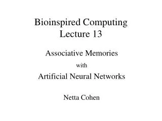
Bioinspired Computing Lecture 9. Artificial Neural Networks: Feed-Forward ANNs Netta Cohen. In Lecture 6….

Bioinspired Computing Lecture 9
E N D
Presentation Transcript
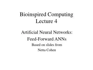
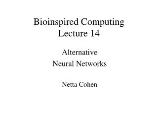
Bioinspired ComputingLecture 9 Artificial Neural Networks: Feed-Forward ANNs Netta Cohen
In Lecture 6… We introduced artificial neurons, and saw that they can perform some logical operations that can be used to solve limited classification problems. We also implemented our first learning algorithm for an artificial neuron. Today • We will build on the single neuron’s simplicity to achieve immense richness at the network level. • We will examine the simplest architecture of feed-forward neural networks and generalise the delta-learning rule to these multi-layer networks. • We look at simple applications and
MP neuron reminder x1 w1 . . . . output xn wn MP neuron (aka single layer perceptron)
1 Activation Flows Forward Hidden 0 input Input Units Output Units Units Error Propagates Backwards The Multi-Layer Network output Step thresholds (which only allow “on” or “off” responses) are replaced by smooth sigmoidal activation functions that are more informative…
Activation Flows Forward Hidden Target Output Input Units Once the error is propagated back, we can solve the credit assignment problem… Units Error Propagates Backwards Backprop Walk-Through… Which of the weights should be changed, and by how much? We need to know which weights contributed most to the error… Output Units Output Units ?
Some definitions & notation… Hidden Units k j z • Binary inputs enter the network through an input layer. For training purposes, inputs are taken from a training set, for which the desired outputs are known. • Neurons (nodes) are arranged in hidden layers & transmit their outputs forward to the output layer. • At each output node, the error: = desired output - actual output. Let desired output =d& Let actual output = oso =d-o. • Label hidden layers, e.g. a,…i,j,k,…; label output layer z. Denote weight on a node in layer k by wjk • After each training epoch, adjust weights by wjk.
Backpropagation in detail • Initialise weights. • Pick rate parameterr. • Until performance is satisfactory: • - Pick an input from the training set • - Run the input through the network & calculate the output. • - For each output node, compare actual output with desired output to find any discrepancies. • - Back-propagate the error to the last hidden layer of neurons (say layer k) as follows: • and repeat for each node in layer k.
r Backpropagation in detail (cont.) • - Continue to back-propagate error, one layer at a time • - Given the errors, compute the corresponding weight changes. For instance, for a node in layer j: • - Repeat for different inputs, • while summing over weight changes for each node. • Update the network. • Halting criterion: typically training stops when a stable minimum is reached in the weight changes, or else when the errors reach an acceptable value (say under 0.1).
Activation Flows Forward Hidden Target Output Input Units ? r Units k Error Propagates Backwards Backprop Walk-Through(take 2) z =dz - oz Output Units Output Units j Iterate until trained...
output hidden bias input bias bias Hidden neurons for curve-fitting after http://users.rsise.anu.edu.au/~nici/teach/NNcourse/ Each hidden unit can be used to represent some feature in our model of the data. Hidden units can be added for additional features. With enough units (and layers), a nnet can fit arbitrarily complex shapes and curves.
How do we train a network? How to choose the learning rate? One solution: adaptive learning rate - The longer we train, the more fine tuned the training, and the slower the rate. How often to update the weights? “batch” learning: the entire training set is run through before updating weights. “online” learning: weights updated with every input sample. Faster convergence possible, but not guaranteed. (Note: Randomise input order for each epoch of training). How to avoid under- and over-fitting?Under- and Over-fitting might occur when the network size or configuration does not match the complexity of the problem at hand.
How do we train a network (cont.) Growing and Pruning: • growing algorithm: • Start with only one hidden unit • If training results in too large an error, add another hidden node. • Continue training & growing the network, until no more improvement is achieved. Pruning: start with a large network & successively remove nodes until an optimal architecture is found. Neurons are assessed for their relative weight in the net & least significant units are removed. Examples of pruning techniques: “optimal brain damage” and “optimal brain surgeon” reflect difficulty in identifying least significant units.
How do we train a network (cont.) Weight decay:Extraneous curvature often accompanies overfitting. Areas with large curvature typically require large weights. Penalising large weights can smooth out the fit. Thus, weight decay helps avoid over-fitting. Training with noise:Add a small random number to each input, so each epoch will look a little different, and the neural net will not gain by overfitting. Validation sets:A good way to know when to stop training the net (i.e. before overfitting) is by splitting the data into a training set and a validation set. Every once in a while, test the network on the validation set. Do not alter the weights! Once the network performs well on both training and validation sets, stop.
Pros and Cons Feed-forward ANNs can overcome the problem of linear separability: Given enough hidden neurons, a feed-forward network can perform any discrimination over its inputs. After a period of training, ANNs can automatically generalise what they learn to new input patterns that they have not yet been exposed to. ANNs are able to tolerate noisy inputs, or faults in their architecture, because each neuron contributes to a parallel distributed process. When neurons fail, or inputs are partially corrupted, ANNs degrade gracefully.
Pros and Cons (cont.) However, unlike the single-unit, the learning algorithm is notguaranteed to find the best set of weight. It may gets stuck at a sub-optimal configuration. Backprop is a form of supervised learning: a “teacher” with all the correct answer must be present, and many examples must be given. Also, unlike Hebbian learning, there is no evidence that backprop takes place in the brain. Feed-forward ANNs are powerful but not entirely natural pattern recognition & categorisation devices…
In 1987 Sejnowski & Rosenberg built a large three-layer perceptron that learned to pronounce English words. The net was presented with seven consecutive characters (e.g., “_a_cat_”) simultaneously as input. NETtalk learned to pronounce the phoneme associated with the central letter (“c” in this example) NETtalk achieved a 90% success rate during training. When tested on a set of novel inputs that it had not seen during training, NETtalk’s performance remained steady at 80%-87%. How did NETtalk work? NETtalkAn early success for feed-forward ANNs
teacher /k/ target output 26 output units 80 hidden units 7 groups of 29 input units 7 letters of text input _ a _ c a t _ target letter The NETtalk Network (after Hinton, 1989)
Initially (with random weights) NETtalk babbled incoherently when presented with English input. As back-propagation gradually altered the weights the target phoneme was produced more and more often. As NETtalk learned pronunciation (e.g., the “a” sound in cat), it generalised this knowledge to other similar inputs: Sometimes this generalisation is useful producing the same sound when it saw the “a” in bat Sometimes it is inappropriate producing the same sound when it saw the “a” in mate After repeated training, NETtalk refined its generalisation, learning to use the context surrounding a letter to correctly influence how the letter was pronounced. NETtalk’s Learning
After learning, NETtalk’s “knowledge” of pronunciation behaves very much like our own in some respects: NETtalk’s Behaviour • NETtalk can generalise its knowledge to new inputs • NETtalk can cope with internal noise & corrupted inputs • When NETtalk fails, its performance degrades gracefully • NETtalk achieves these useful abilities automatically. • In contrast, a programmer would have to work very hard to equip a standard database with them. • NETtalk’s knowledge is robust and flexible • A database is fragile and brittle • What does NETtalk’s knowledge look like?
Each hidden neuron in the net is used to detect a different feature of the input. These features were then used to divide up the input space into useful regions. By detecting which regions an input falls within, the net can tell whether it should return 1 or return 0. NETtalk’s Hidden Unit Subspaces NETtalk uses the same trick. It uses the hidden units to detect 79 different features… In other words, its weights divide its input space into 79 regions There are 79 regions because there are 79 English letter-to-phoneme relationships. Examining the weights allows us to cluster these features/regions, grouping similar ones together…
How sophisticated is NETtalk’s knowledge? Does NETtalk possess the concept of a “vowel” or a “\k\”? No – NETtalk can only use its knowledge in a fixed and limited way. Philosophers have imagined that concepts resemble Prolog propositions. They are distinct, general-purpose, logical, and symbolic. They represent facts in the same way that English sentences do and can enter into any kind of reasoning or logic. They are part of the language of thought… In contrast, NETtalk’s knowledge is more like a skill: Muddled together, special purpose, not logical or symbolic. More on this distinction later… NETtalk’s Knowledge
A Vision Application Hubert & Wiesel’s work on cat retinae has inspired a class of ANNs that are used for sophisticated image analysis. Neurons in the retina are arranged in large arrays, and each has its own associated receptive field. How does this arrangement enable pattern formation? One key component is edge detection based on lateral inhibition. An ANN can do the same thing: A pattern of light falls across an array of neurons that each inhibit their right-hand neighbour. Only neurons along the left-hand dark-light boundary escape inhibition. Lateral inhibition such as this is characteristic of natural retinal networks. Now let the receptive fields of different neurons be coarse grained, with large overlaps between adjacent neurons. What advantage is gained?
Distributed Representations In the examples today, nnets learn to represent the information in a training set by distributing it across a set of simple connected neuron-like units. • Some useful properties of distributed representations: • they are robust to noise • they degrade gracefully • they are content addressable • they allow automatic completion orrepair of input patterns • they allow automatic generalisation from input patterns • they allow automatic clustering of input patterns In many ways, this form of information processing resembles that carried out by real nervous systems.
Distributed Representations However, distributed representations are quite hard for us to understand, visualise or build by hand. • To aid our understanding we have developed various ideas: • the partitioning of the input space • the clustering of the input data • the formation of feature detectors • the characterisation of hidden unit subspaces • etc. To build distributed representations automatically, ANNs resort to learning algorithms such as backprop.
Problems ANNs often depart from biological reality: Supervision: Real brains cannot rely on a supervisor to teach them, nor are they free to self-organise. Training vs. Testing: This distinction is an artificial one. Temporality: Real brains are continuously engaged with their environment, not exposed to a series of disconnected “trials”. Architecture: Real neurons and the networks that they form are far more complicated than the artificial neurons and simple connectivity that we have discussed so far. Does this matter? If ANNs are just biologically inspired tools, no, but if they are to model mind or life-like systems, the answer is maybe.
Problems Problems Fodor & Pylyshyn raise a second, deeper problem, objecting to the fact that, unlike classical AI systems, distributed representations have no combinatorial syntactic structure. Cognition requires a language of thought. Languages are structured syntactically. If ANNs cannot support syntactic representations, they cannot support cognition. F&P’s critique is perhaps not a mortal blow, but is a severe challenge to the naive ANN researcher…
Next Lecture on this topic… • More neural networks… • More learning algorithms... • More distributed representations... • How neural networks deal with temporality. Reading • Follow the links in today’s slides. • In particular, much of today was based on • http://www.idsia.ch/NNcourse/intro.html