ITEC452 Distributed Computing Lecture 9 Graph Algorithms
Hwajung Lee. ITEC452 Distributed Computing Lecture 9 Graph Algorithms. Graph Algorithms. Why graph algorithms ? It is not a “graph theory” course! Many problems in networks can be modeled as graph problems. Note that - The topology of a distributed system is a graph .


ITEC452 Distributed Computing Lecture 9 Graph Algorithms
E N D
Presentation Transcript
Hwajung Lee ITEC452Distributed ComputingLecture 9Graph Algorithms
Graph Algorithms Why graph algorithms ? It is not a “graph theory” course! Many problems in networks can be modeled as graph problems. Note that - The topology of a distributed system is a graph. - Routing table computation uses the shortest path algorithm - Efficient broadcasting uses a spanning tree - Maxflow algorithm determines the maximum flow between a pair of nodes in a graph.
Routing • Shortest path routing • Distance vector routing • Link state routing • Routing in sensor networks • Routing in peer-to-peer networks
Internet routing Autonomous System Autonomous System AS1 AS0 Each AS is under a common administration Autonomous System Autonomous System AS2 AS3 Intra-AS vs. Inter-AS routing Shortest Path First routing algorithm is the basis for OSPF
Routing revisited (borrowed from Cisco documentation http://www.cisco.com)
Routing: Shortest Path Most shortest path algorithms are adaptations of the classic Bellman-Ford algorithm. Computes shortest path if there are no cycle of negative weight. Let D(j) = shortest distance of j from initiator 0. Thus D(0) = 0 w(0,m),0 0 m j (w(0,j)+w(j,k)), j The edge weights can represent latency or distance or some other appropriate parameter. k Classical algorithms: Bellman-Ford, Dijkstra’s algorithm are found in most algorithm books. What is the difference between an (ordinary) graph algorithm and a distributed graph algorithm?
Shortest path Revisiting Bellman Ford : basicidea Consider a static topology Process 0 sends w(0,i),0 to neighbor i {program for process i} do message = (S,k) S < D(i) if parent ≠ k parent := k fi; D(i) := S; send (D(i)+w(i,j),i) to each neighbor j ≠ parent; message (S,k) S ≥ D(i) --> skip od Current distance Computes the shortest distance to all nodes from an initiator node The parent pointers help the packets navigate to the initiator
Shortest path Chandy & Misra’s algorithm : basic idea Consider a static topology Process 0 sends w(0,i),0 to neighbor i {for process i > 0} do message = (S ,k) S < D if parent ≠ k send ack to parent fi; parent := k; D := S; send (D + w(i,j), i) to each neighbor j ≠ parent; deficit := deficit + |N(i)| -1 message (S,k) S ≥ D send ack to sender ack deficit := deficit – 1 • deficit = 0 parent i send ack to parent od 0 2 1 7 1 2 3 2 4 7 4 2 6 6 5 3 Combines shortest path computation with termination detection. Termination is detected when the initiator receives ack from each neighbor
Shortest path An important issue is: how well do such algorithms perform when the topology changes? No real network is static! Let us examine distance vector routing that is adaptation of the shortest path algorithm
Distance Vector Routing Distance Vector D for each node i contains N elements D[i,0], D[i,1], D[i,2] … Initialize these to {Here, D[i,j] defines its distance from node i to node j.} - Each node j periodically sends its distance vector to its immediate neighbors. - Every neighbor i of j, after receiving the broadcasts from its neighbors, updates its distance vector as follows: k≠ i: D[i,k] = mink(w[i,j] + D[j,k] ) Used in RIP, IGRP etc 1 1 1 1 D[j,k]=3 means j thinks k is 3 hops away
Counting to infinity Observe what can happen when the link (2,3) fails. Node1 thinks d(1,3) = 2 Node 2 thinks d(2,3) = d(1,3)+1 = 3 Node 1 thinks d(1,3) = d(2,3)+1 = 4 and so on. So it will take forever for the distances to stabilize. A partial remedy is the split horizon method that will prevent 1 from sending the advertisement about d(1,3) to 2 since its first hop is node 2 k≠ i: D[i,k] = mink(w[i,j] + D[j,k] ) Suitable for smaller networks. Larger volume of data is disseminated, but to its immediate neighbors only Poor convergence property
Link State Routing Each node i periodically broadcasts the weights of all edges (i,j) incident on it (this is the link state) to all its neighbors. The mechanism for dissemination is flooding. This helps each node eventually compute the topology of the network, and independently determine the shortest path to any destination node using some standard graph algorithm like Dijkstra’s. Smaller volume data disseminated over the entire network Used in OSPF
Link State Routing • Each link state packet has a sequence numberseq that determines the order in which the packets were generated. • When a node crashes, all packets stored in it are lost. After it is repaired, new packets start with seq = 0. So these new packets may be discarded in favor of the old packets! • Problem resolved using TTL
Complexity of Bellman-Ford Theorem. The message complexity of Bellman-Ford algorithm is exponential. Proof outline. Consider a topology with an even number nodes 0 through n-1 (the unmarked edges have weight 0) n-4 n-2 1 3 5 20 2k 2k-1 22 21 n-5 n-3 n-1 0 4 2 Time the arrival of the signals so that D(n-1) reduces from (2k+1- 1) to 0 in steps of 1. Since k = (n-1)/2, it will need 2(n+1)/2-1 messages to reach the goal. So, the message complexity is exponential.
Interval Routing (Santoro and Khatib) Conventional routing tables have a space complexity O(n). Can we route using a “smaller” routing table? Yes, by using interval routing. This is the motivation.
Interval Routing: Main idea • Determine the interval to which the destination belongs. • For a set of N nodes 0 . . N-1, the interval [p,q)between p and q (p, q < N) is defined as follows: • if p < q then [p,q) = p, p+1, p+2, .... q-2, q-1 • if p ≥ q then [p,q) = p, p+1, p+2, ..., N-1, N, 0, 1, ..., q-2, q-1 [5,1) [3,5) [1,3)
Example of Interval Routing N=11 Labeling is the crucial part
Labeling algorithm Label the root as 0. Do a pre-order traversal of the tree. Label successive nodes as 1, 2, 3 For each node, label the port towards a child by the node number of the child. Then label the port towards the parent by L(i) + T(i) + 1 mod N, where - L(i) is the label of the node i, - T(i) = # of nodes in the subtree under node i (excluding i), Question 1. Why does it work? Question 2. Does it work for non-tree topologies too? YES, but the construction is somewhat tricky.
Anotherexample Interval routing on a ring. The routes are not optimal. To make it optimal, label the ports of node i with i+1 mod 8 and i+4 mod 8.
Example of optimal routing Optimal interval routing scheme on a ring of six nodes
So, what is the problem? Works for static topologies. Difficult to adapt to changes in topologies. But there is some recent work on compact routing in dynamic topologies (Amos Korman, ICDCN 2009)
Prefix routing Easily adapts to changes in topology, and uses small routing tables, so it is scalable. Attractive for large networks, like P2P networks. a b When new nodes are added or existing nodes are deleted, changes are only local. a.a.a a.a.b
Another example of prefix routing destination 130102 source 203310 13010-1 1301-10 Pastry P2P network 130-112 13-0200 1-02113
Spanning tree construction For a graph G=(V,E), a spanning tree is a maximally connected subgraph T=(V,E’), E’ E,such that if one more edge is added, then the subgraph is no more a tree. Used for broadcasting in a network with O(N) complexity. Chang-Robert’s algorithm {The root is known} {main idea} Uses probes and echoes, and keeps track of deficits C and D as in Dijkstra-Scholten’s termination detection algorithm first probe --> parent: = sender; C=1 forward probe to non-parent neighbors; update D echo --> decrement D probe and sender ≠ parent --> send echo C=1 and D=0 --> send echo to parent; C=0 Parent pointer Question:What if the root is not designated?
Graph traversal Think about web-crawlers, exploration of social networks, planning of graph layouts for visualization or drawing etc. Many applications of exploring an unknown graph by a visitor (a token or mobile agent or a robot). The goal of traversal is to visit every node at least once, and return to the starting point. - How efficiently can this be done? - What is the guarantee that all nodes will be visited? - What is the guarantee that the algorithm will terminate? DFS (or BFS) traversal is well known, so we will not discuss about it
Graph traversal Tarry’s algorithm is one of the oldest (1895) Rule 1. Send the token towards each neighbor exactly once. Rule 2. If rule 1 is not applicable, then send the token to the parent. A possible route is: 0 1 2 5 3 1 4 6 2 6 4 1 3 5 2 1 0 Nodes and their parent pointers generate a spanning tree.
Minimum Spanning Tree Given a weighted graph G = (V, E), generate a spanning tree T = (V, E’) E’ E such that the sum of the weights of all the edges is minimum. Applications Minimum cost vehicle routing On Euclidean plane, approximate solutions to the traveling salesman problem, Lease phone lines to connect the different offices with a minimum cost, Visualizing multidimensional data (how entities are related to each other) We are interested in distributed algorithms only The traveling salesman problem asks for the shortest route to visit a collection of cities and return to the starting point.
Sequential algorithms for MST Review (1) Prim’s algorithm and (2) Kruskal’s algorithm. Theorem. If the weight of every edge is distinct, then the MST is unique.
Minimum Spanning Tree Given a weighted graph G = (V, E), generate a spanning tree T = (V, E’) such that the sum of the weights of all the edges is minimum. Applications On Euclidean plane, approximate solutions to the traveling salesman problem, Lease phone lines to connect the different offices with a minimum cost, Visualizing multidimensional data (how entities are related to each other) We are interested in distributed algorithms only The traveling salesman problem asks for the shortest route to visit a collection of cities and return to the starting point.
Sequential algorithms for MST Review (1) Prim’s algorithm and (2) Kruskal’s algorithm. Theorem. If the weight of every edge is distinct, then the MST is unique.
Gallagher-Humblet-Spira (GHS) Algorithm • GHS is a distributed version of Prim’s algorithm. • Bottom-up approach. MST is recursively constructed by fragments joined by an edge of least cost. 3 7 5 Fragment Fragment
Challenges Challenge 1. How will the nodes in a given fragment identify the edge to be used to connect with a different fragment? A root node in each fragment is the root/coordinator
Challenges • Challenge 2. How will a node in T1 determine if a given edge connects to a node of a different tree T2 or the same tree T1? Why will node 0 choose the edge e with weight 8, and not the edge with weight 4? • Nodes in a fragment acquire the same name before augmentation.
Two main steps • Each fragment has a level. Initially each node is a fragment at level 0. • (MERGE) Two fragments at the same level L combine to form a fragment of level L+1 • (ABSORB) A fragment at level L is absorbed by another fragment at level L’ (L < L’). The new fragment jhas a level L’. (Each fragment in level L has at least 2L nodes)
Least weight outgoing edge To test if an edge is outgoing, each node sends a test message through a candidate edge. The receiving node may send accept or reject. Rootbroadcastsinitiate in its own fragment, collects the report from other nodes about eligible edges using a convergecast, and determines theleast weight outgoing edge. test accept reject
Accept of reject? Let i send test to j Case 1. If name (i) = name (j) then send reject Case 2. If name (i)≠name (j) level (i)level (j) then send accept Case 3. If name (i) ≠ name (j) level (i) > level (j) then wait untillevel (j) = level (i) and then send accept/reject. WHY? (Note that levels can only increase). Q: Can fragments wait for ever and lead to a deadlock? reject test test
The major steps repeat • Test edges as outgoing or not • Determine lwoe - it becomes a tree edge • Send join (or respond to join) • Update level & name & identify new coordinator/root until done
Classification of edges • Basic (initially all branches are basic) • Branch (all tree edges) • Rejected (not a tree edge) Branch and rejected are stable attributes
Wrapping it up Example of merge Merge The edge through which the join message is exchanged, changes its status to branch, and it becomes a tree edge. The new root broadcasts an (initiate, L+1, name) message to the nodes in its own fragment. initiate
Wrapping it up Absorb T’ sends a join message to T, and receives an initiate message. This indicates that the fragment at level L has been absorbed by the other fragment at level L’. They collectively search for the lwoe. The edge through which the join message was sent, changes its status to branch. initiate Example of absorb
Example 8 0 2 1 5 1 3 7 4 5 4 6 2 6 3 9
Example 8 merge merge 0 2 1 5 1 3 7 4 5 4 6 2 merge 6 3 9
Example 8 0 2 1 5 1 7 merge 3 4 5 4 6 absorb 2 6 3 9
Example absorb 8 0 2 1 5 1 7 3 4 5 4 6 2 6 3 9
Message complexity At least two messages (test + reject) must pass through each rejected edge. The upper bound is 2|E| messages. At each of the log N levels, a node can receive at most (1) one initiate message and (2) one accept message (3) one join message (4) one test message not leading to a rejection, and (5) one changeroot message. So, the total number of messages has an upper bound of 2|E| + 5N logN