Spurs in HIFI data
110 likes | 290 Views
Spurs in HIFI data. Artifacts in HIFI Data. Generally, there are three major cleaning exercises with HIFI data. Baseline subtraction Standing Wave removal Spur flagging In this talk/demo, we concentrate on spurious response in HIFI. Spur Definition and Detection.

Spurs in HIFI data
E N D
Presentation Transcript
Artifacts in HIFI Data • Generally, there are three major cleaning exercises with HIFI data. • Baseline subtraction • Standing Wave removal • Spur flagging • In this talk/demo, we concentrate on spurious response in HIFI.
Spur Definition and Detection For the purposes of this discussion, we define spurs as those features which are generally Gaussian in shape and narrow (<50MHz). They can look like astronomical lines, and have the potential to ‘fool’ users.
Related artifacts Other artifacts due to saturated detectors or under pumped mixers can also corrupt HIFI spectra, but are much more obvious and easy to remove.
Spur Detection in HIFI SPG • Because spurs can look like real lines, we search for them only in the loads. The algorithm used in the standard HIFI pipeline is as follows: • Loop through each WBS HTP at level 0.5 • Loop through each cold load within this HTP • Loop through each subband in the load dataset • Flag saturated pixels • Compute second derivative of the load spectrum • Mark points in the 2nd derivative that exceed a threshold and fit as a spur. • Flag the spur, and record parameters in a table (trend analysis section of obs context). As part of the level 0.5->level 1 pipeline, flux calibration is performed and as a result flags in the loads are propagated naturally to the science data.
The obs context spur table obs=getObservation("134281161” ,poolName="1342181161_sscan_dbs_1b_r4")
The obs context spur table obs=getObservation("134281161” ,poolName="1342181161_sscan_dbs_1b_r4")
HSPOT and Spur Reporting Based on repeated observations, we find that spur positions (LO vs IF) are generally stable and repeatable. Weak spurs (in particular band 4b) can come and go based on the conditions of the instrument at the time of observation. This means we warn users at the HSPOT planning stage if their observation is in danger of being corrupted by a spur.
Diverse Spur Behavior Strong spurs, such as the (now fixed) spur in 1a, can knock out an entire dataset. Weak spurs can impact only a very narrow region (4b for example) Some spurs have a predictable position in the IF as a function of the LO frequency.
More spur pathology Some spurs can move in IF over time. If an observation goes on a long time before a LO retune, the spur can ‘migrate’ out of the flagged region and complicate data reduction (most notably for spectral scans). Spurs can be missed by the algorithm if the load is not as ‘smooth’ as expected. Such data need to be flagged manually, and we discuss this in the demo.
Spur impact on deconvolution Historically, the spur finder was developed for use in spectral surveys, where artifacts such as these can significantly corrupt the result from the deconvolution. It has now matured into a full featured, automated pipeline module for ALL observations, regardless of mode. Deconvolved output from data with an unflagged spur. The iterative nature of the algorithm propagates the spur over the entire spectral range. Same spectrum, this time with the spur masked out. The result reveals some baseline issues that now need to be addressed. Final result after simple median baseline subtraction.