Download
1 / 11
110 likes | 242 Views
HIFI Spectral Maps in HIPE. Pat Morris, NHSC DP Webinar, 9 March 2012. Organization and Goals. Part I: Some information relevant to this webinar about spectral map processing and basic analysis in HIPE Part II: 8-part Scripted Demo

E N D
HIFI Spectral Maps in HIPE Pat Morris, NHSC DP Webinar, 9 March 2012
Organization and Goals • Part I: Some information relevant to this webinar about spectral map processing and basic analysis in HIPE • Part II: 8-part Scripted Demo • Data inspection, identification of artifacts that can affect map data quality • Artifact treatments • Merging products to achieve best S/N ratios • The doGridding task for cube generation, using default and tuned parameters • The Cube Spectrum Analysis Toolbox (CSAT) • Some useful Image Analysis tools (mainly where to find them)
Logistics • Data and scripts are on the NHSC webdav, please refer to https://nhscsci.ipac.caltech.edu/sc/index.php/Hifi/HIFIWebinarPreparations • The main demo script is called MappingDemoHIFIDPWSMar2012.py. • Highly annotated in tutorial fashion. • You are not expected to follow along step by step • I will proceed at a pace to allow you to understand what I am doing, ask questions, and try on your own either during the demo or afterwards. • The session will be recorded, edited, and posted for reference. • Due to time and scope, I do not give an overview of HIFI’s spectral mapping AOT and the various OTF and DBS Raster modes. • If you do not have your own program data and/or familiarity with the mapping modes, please visit the HIFI Calibration Web http://herschel.esac.esa.int/twiki/bin/view/Public/HifiCalibrationWeb • HIFI Observers Manual version 2.4 • HIFI AOT Performance Notes version 3.0
HIPE and exo-HIPE • HIPE version is 8.1, however… • A bug is present in a certain part of the CSAT which I will point out. In order to conduct the demo without a workaround for this bug, I will be using HIPE 8.2 (internal build 8.0.3452). It will barely affect you today. The User Release version of this is due any day. • We will work in HIPE. Also… • I recommend having an HSpot session open, to examine the AOR setups and visualizations. • Using DS9 or your favorite FITS viewer is helpful. • IDL, CLASS, other environments may be preferred by some users, but not today (I will not be moving between these environments). • In HIPE we will use the Spectrum Explorer and CSAT. Be aware that in HIPE 9, these two environments are planned to be merged (CSAT Spectrum Explorer = SE-II). TBC, currently in heavy development.
Tour of HIFI Map Data (1) Data products loaded from a pool in my local store area are registered in the variable I called “obs” which is an observation context (obsContext in HIPE speak), not unlike data from other HIFI observation modes.
Tour of HIFI Map Data (2) Under the level2 products: Calibrated HIFI Timeline Products (HTPs) by spectrometer, polarization, and sideband Spectral cubes produced in the level2 pipeline. In HIPE 9 the doGridding task that creates the spectral cubes will be part of a new level2.5 pipeline, and cube products will be found under level2.5
Tour of HIFI Map Data (3) The “cubes” folder is a MapContext that contains all of the generated spectral cube products. A cube has been created for each level2 HTP, but also by spectrometer sub-band. Cubes on a sub-band basis are historically to keep out artifacts of different sub-band calibration offsets (not really an issue), and to control memory utilization. This can still be a problem for large spectral maps, and the user can create maps for one spectrometer, one polarization, one sideband, and one sub-band at a time. However, the user can create cubes of all sub-bands at once, using the doStich task on the input HTP(s). This can be an advantage for lines with straddle sub-bands in the IF.
Tour of HIFI Map Data (4) Inside each cube product are the image data and weighting by spectral dataset that was convolved into the cube. If the image product is clicked, it is displayed with the Image Viewer for Array Datasets. This viewer is used in Spectrum Explorer when opened on cubes, and the CSAT. Also the associated WCS is shown. The scroll bar allows you to scroll through each of the channels corresponding to a calibrated frequency.
Tour of HIFI Map Data (5)The HifiUplinkProduct Starting in HIPE 8.0, a HifiUplinkProduct will appear under the Auxiliary tree of the obs context. It contains AOR setup and performance predictions from HSpot time estimation at the time of scheduling. These parameters are needed in the pipeline, and by the user to compare observed and predicted noise levels. This product cannot be created in HIPE, needs to be created from level “-1”, at the telemetry and dataframe assembly level. So, by bulk reprocessing at HSC, or On-Demand reprocessing in the HSA starting in HIPE 9.0. The contents of the HifiUplinkProduct will contain the AOR performance parameters (actual map dimensions, noise predictions, etc) for observations starting with obsid 1342227385. For earlier observations (such as this example), only the requested AOR parameters are present. Backfilling is underway.
A note about doGridding in HIPE 7 and later • Starting in HIPE 7 the doGridding task was modified to more directly use on the actual uplink parameter (from HSpot time estimation) output of the map dimensions (scan leg and readout separation), or to set the default sampling and WCS of the spectral cubes (effectively the pixel sizes). • It also uses a modified approach when those parameters are not present in the obs products (UplinkProduct or HifiUplinkProduct), reconstructing from pointing assignments to the spectral data. • This provides the default cube construction which most closely matches how the map was executed, and provides the basis for browse products. • Data processed < SPG 7.0 should be reprocessed in the pipeline starting at level1, either in HIPE or with the On Demand reprocessing in the HSA. • A script is provided on the webdav.
Questions? 835 GHz continuum