Download
1 / 13
130 likes | 291 Views
Tour of HIFI data. Outline. Opening the observation context Straight to the ‘science’ result (level 2) A casual look at the HIPE GUI presentation of your data The HISTORY section. The AUXILIARY section The CALIBRATION section The QUALITY section The Trend Analysis section

E N D
Outline • Opening the observation context • Straight to the ‘science’ result (level 2) • A casual look at the HIPE GUI presentation of your data • The HISTORY section. • The AUXILIARY section • The CALIBRATION section • The QUALITY section • The Trend Analysis section • A review of how DBS observations work
Opening the observation context Within HIPE, open and run the ‘tour_of_hifi_data.py’ script. Alternatively you can type the following in your console: obsP=getObservation("1342190183” \ ,poolName="1342190183_point_fastdbs_1b") TIP: the ‘\’ in the above lets you type long commands in HIPE by spanning them over a several lines.
The HIPE GUI and your data • The HIPE display for an observation context is a lot like a graphical file system listing. In this analogy, directories are what we call ‘Products’, and the files in directories called ‘datasets’. • Products can contain other products, just like a directory can have subdirectories. • The GUI is broken up into a tree listing (side), a summary/meta data description (top), and a dataset display tool (right) • Used properly, the GUI can be very powerful in letting you navigate and assess the quality and content of your data.
HIFI Observation Contexts • The observation context contains everything you need to reprocess your data. Pointing data, calibration files, and raw data are all contained in different parts of the tree. • The caveat to this is that if new calibration information is uploaded to HSA, one needs to fetch it first before (or during) any reprocessing. • The different ‘levels’ of data denote various levels of processing. Level 0 is the raw data, while Level 2 is fully calibrated and corrected for spacecraft motion.
HISTORY SECTION • Most users will not use this section. It contains an accounting of what tasks were run to process the data, and what the parameters were. • In general the tasks are always going to be ‘xxxPipeline’
AUXILIARY Section • This section contains an abundance of pointing information, and in general is far beyond what users need to to worry about. • The ‘EventsLogProduct’ contains a listings of anomalies that were flagged during the time your data was taken. In general there will be a lot of them, and can be safely ignored. • One section that users may refer to more often is the ‘UplinkProduct’, which contains details from your proposal and AOR settings.
The CALIBRATION Section • This section contains a set of static tables stored at the HSA, as well as calibration related information determined during processing of the data. • Sideband gains, the efficiencies, and so on are stored in the DOWNLINK part of the table. The user, if they so wish, can modify these tables manually and repipeline their data using the new values. • A list of bad pixels, Tsys measurements from the loads, etc, are stored in the PIPELINE-OUT section. Changes made here will, in general, get overwritten if the user repipelines their data.
The QUALITY Section • Although the tree stores a lot of information (much of which is admittedly opaque to the general user), the topmost level summary is the best way to quickly assess your data • Critical items will be highlighted in color, though in most cases the quality section is populated mainly with warning messages that can be safely ignored.
The TREND ANALYSIS Section • Everything in this section is derived from measurements of the data in the current observation context. • It stores the fits to the comb observations (frequency calibration), estimates of the Tsys based on the load observations, and also a table of spurs or other spectral anomalies found in the data (more on this in the SPUR presentation).
The HifiTimelineProduct • Within each data ‘level’, the tree is broken up into sections for the four backends. • For each backend, data is stored in what we call a “HifiTimelineProduct”, or HTP. Within a HTP, spectra are stored in the order they are taken. • The best way to examine the order is via the SUMMARY TABLE. • The BBID indicates what type of observation is being done. • The ‘isLine’ flag is TRUE when the primary beam is on target. • isHRS and isWBS indicate when those backends are collecting data • ‘length’ tells you how many spectra were obtained for that cycle.
DBS Observations POSITION Ref 2 Position 1 NOD 1 2 180” chop throw TIME 3 NOD 2 4 Ref 1 Position 180” chop throw (1-2) + (4-3) Target Position
A teaser for later • At level 1 the data have been flux calibrated. In the data used for this demo, it is interesting to compare spectra obtained from each of the two NOD positions. • To do this, navigate to the WBS-H part of the level 1 tree. By inspecting the summary table, we can tell that dataset #4 corresponds to data taken at nod position 1, and dataset #5 from position 2. • Navigate to these data and drag them to the VARIABLES tab. Rename them if you like. • Double click on the first one to plot it, then drag the second on top of the plot so they are overlaid. Note the difference! This is due to emission in the reference position, and cleaning that up is a topic of another talk later today.