Download
1 / 23
230 likes | 244 Views
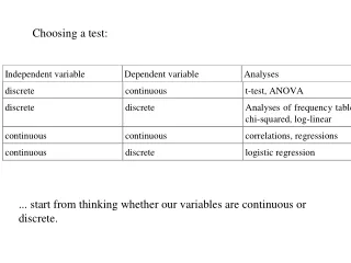
Choosing a test:. ... start from thinking whether our variables are continuous or discrete. The power of a test is the probability that the test finds a statistically significant effect ... .... in case the effect of certain strength actually occurs in the population.

E N D
Choosing a test: ... start from thinking whether our variables are continuous or discrete.
The power of a test is the probability that the test finds a statistically significant effect... ....in case the effectof certain strength actually occurs in thepopulation. - can be used in two situations - planning experiments – how large sample to take? - concluding from negative results. A non-significant result as such is not a strong argument. We can never prove that there is no relationship!
But we can show that the strength of the relationship is not larger than .... (some biologically relevantvalue), • we could not show statistical significance, but if the relationship would have been as strong as ..., would it have been very likely (e.g. 84,5% - this is the power!) to get it significant, but as we did not, then probably there still isn’t that strong relationship in the populations. An easier way – confidence limits to parameters.
Hypotheses testing: null hypothesis and research hypothesis: HO: - there is no difference; H1: - there is a difference; Type I error: declare H1 correct, when it actually isn’t; Type II error: remain with HO, although H1 is actually correct. Conservative tests have lower type I error risk but have higher risk of type II error.
Information criteria in model selection, AIC – Akaike Information Criterion, IT-approach; ... simplifying model, which independent variables to include/ drop? ... in situations in which we wish to sort out determinants of our independent variable, especially on the landscape, occurence of a species, especially when we want to predict. Entire models (sets of independent variables) are compared - the models as such get points; - not based on p-values of particular variables;
We can compare the models on the basis of AIC values, AIC score depends on: - model fit (likelyhood); - complexity of the model; the model with lowest AIC is declared the best! Model fit... also R-square but that is always larger for more complex models; in AIC approach, the models get punished for their complexity; did increasing the complexity improve its fit much enough to justify it?
What does the abundance of toads depend on? - abundance of slugs; - abundance of earthworms; - density of pools. Slugs Worms Pools error
Two ways how to make conclusions: • the best model (smallest AIC); • model averaging: a set of „good“ models is found, they • get weights according to AIC values; • for particular independent variables, importances can • be calculated, according to presence of the variable in • good models; • ... the variables get more importance points for being present • in better models; • .... variables can be ranked according to their importance.
Occurrence of Phengaris arion on Saaremaa island, Margus Vilbas et al. 2015
Bayesian statistics, ... we have a sample and a priori information about which value of a variable is how likely to occur; ... in ordinary statistics we have only sample; .... we change our prior understanding based on our sample; ... we have a positive relationship with 99% probability = there is 1 % probability that there is not = the positive relationship in our sample was obtained by chance with 1% probability; .... the ordinary p-value cannot be interpreted this way!
Bayesian statistics in more detail .... a gambler gets „six“ throwing a dice, …. ordinary dice vs. cheating dice; .... for ordinary dice, the probability is 16,7%, this is p. … this is the probability to get „6“ by chance, this is p. … but it is not the probability that „6“ was got by chance (= probability, that the dice is OK); ... 16,7% is not the probability that the dice is OK, we do not know...
But if we know in advance, that in half of the cases, the gambler uses the cheating dice, we can calculate, that the probability of having a cheating dice today is 85,7%, vs 14,3% for the ordinary dice. This 50:50 is prior distribution; 85,7:14,3 is our posterior distribution. Posterior distribution depends 1) on prior distrobution; 2) on our sample.
The gambler gets „six“, the probability that he has a cheating dice depends on - probability to get „6“ using ordinary dice; - probability that cheating dice is used; We have caught 6 female and 10 male bears from the forest, we can calculate the probability of getting this by chance if in the population there is 1:1 ratio; this is p; - we need to know only the sample; .... to answer the question „how likely it is that our population is female biased?“, we must know the probability of the occurrence of such populations in nature. If female-biased populations are very rare, it is much more likely that we just got an odd sample from a male-biased population.
There is a significant relationship in one group but there was not a significant relationship in another? We study the effect of fertilisation on the growth of birch and aspen, two treatments (fertilised or not), dependent variable is three height. For aspen, an effect of fertilisation was found (p = 0,01), but not for birch (p = 0,08). can we say that there is a (statistically significant) difference in the effect of fertiliser between the tree species?
No we cannot. We have to test the treatment*species interaction! aspen sign effect effect strength birch zero effect
If to be absolutely honest, then we should have the hypothesis before looking at the data p value for the hypothesis that last lecture of this course happens on 19th? Null hypothesis and research hypothesis: HO: last statistics lecture happens on whatever date; H1: last statistics lecture happens on 19th day of a month; p = ???
.... p value for the hypothesis that last lecture of this course happens on 19th? p = 1/30 = 0,0333 Is it then statistically significant, that on 19th day of a month? No, because we set up or hypothesis looking at our data, the hypothesis should be independent of the data.
statistics does not answer the question • about causality; • do not divide a continuous variable into • classes for the analysis, • but you can do so in a figure;
„Nothing reveals mathematical illiteracy better than excessive accuracy in calculations “.