Download
1 / 39
390 likes | 472 Views
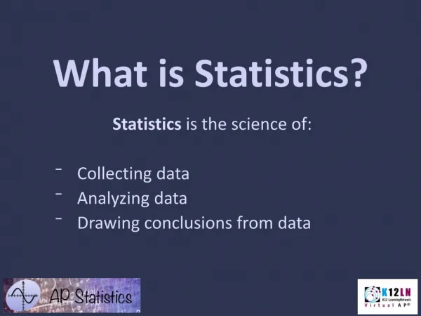
Learn about ratio, interval, ordinal, and nominal scales, precision, accuracy, significant figures in measurements, and rules for rounding in basic statistics lessons.

E N D
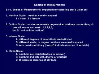
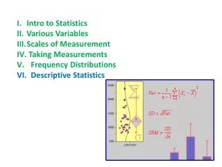
Intro to Statistics • Various Variables • Scales of Measurement
Intro to Statistics • Various Variables • Scales of Measurement • A. Data on a ratio scale • Data on a ratio scale have a constant and defined unit of measurement that assigns a real number to all measurements. • Such data has a constant size interval between any adjacent units on the measurement scale. • A zero point on the measurement scale must exist and there must be a physical significance to this zero. • Ratio scales include things like mass, length, number, volumes, lengths of time, etc.
Intro to Statistics • Various Variables • Scales of Measurement • A. Data on a ratio scale • B. Data on an interval scale • Same as ratio scale, except that in an interval scale no true zero exists on the measurement scale – it is ‘arbitrary’ • Example - temperature on the Celsius or Fahrenheit scales.
Intro to Statistics • Various Variables • Scales of Measurement • A. Data on a ratio scale • B. Data on an interval scale • C. Data on an ordinal scale • This scale uses ranked variables.
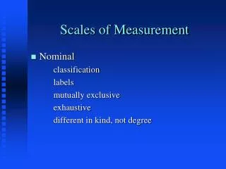
Intro to Statistics • Various Variables • Scales of Measurement • A. Data on a ratio scale • B. Data on an interval scale • C. Data on an ordinal scale • D. Data on a nominal scale • This ‘scale’ uses attributes. Thus even relationships like greater than or less than don’t apply
Intro to Statistics • Various Variables • Scales of Measurement • Taking Measurements • A. Precision and Accuracy • Accuracy– the closeness of a measured or computed value to its true value
Intro to Statistics • Various Variables • Scales of Measurement • Taking Measurements • A. Precision and Accuracy • Accuracy– the closeness of a measured or computed value to its true value • Precision– the closeness of repeated measurements of the same quantity to each other
Intro to Statistics • Various Variables • Scales of Measurement • Taking Measurements • A. Precision and Accuracy • How accurate? • 30-300 rule. • Range should be about 30-300 unit steps. • Length of shells 4-9mm? 4 units steps. • 4.2-9.4? 52 unit steps.
Intro to Statistics • Various Variables • Scales of Measurement • Taking Measurements • A. Precision and Accuracy • B. Significant Figures http://www.chem.sc.edu/faculty/morgan/resources/sigfigs/index.html
All nonzero digits are significant: 1.234 g has 4 significant figures, 1.2 g has 2 significant figures. • (2) Zeroes between nonzero digits are significant: • 1002 kg has 4 significant figures, 3.07 mL has 3 significant figures. • (3) Leading zeros to the left of the first nonzero digits are not significant • 0.001 g has only 1 significant figure ….change unit! = 1 mg(4) Trailing zeroes to the right of a decimal point in a number are significant: • 0.0230 mL has 3 significant figures,(5) When a number ends in zeroes that are not to the right of a decimal point, the zeroes are not necessarily significant: • 190 miles may be 2 or 3 significant figures, 50,600 calories may be 3, 4, or 5 significant figures. • (6) EXACT numbers, often integers (counts) – infinite sig figs • The potential ambiguity in the last rule can be avoided by the use of standard exponential, or "scientific," notation, or a change in the unit. For example, depending on whether the number of significant figures is 3, 4, or 5, we would write 50,600 calories as: • 5.06 × 10⁴ calories (3 significant figures) 5.060 × 10⁴ calories (4 significant figures), or 5.0600 × 10⁴ calories (5 significant figures). From Morgan 2012
Mathematical Operations: When adding/subtracting: last common digit farthest to right: 100 (assume 3 significant figures) + 23.643 (5 significant figures) = 123.643 (124) When multiplying/dividing: same as one with smallest number of sig. figs. 3.0 (2 significant figures ) × 12.60 (4 significant figures) = 37.8000 (38) Carry all numbers and round at the end: In a long calculation involving mixed operations, carry as many digits as possible through the entire set of calculations and then round the final result appropriately. For example, (5.00 / 1.235) + 3.000 + (6.35 / 4.0)=4.04858... + 3.000 + 1.5875=8.630829... The first division should result in 3 significant figures. The last division should result in 2 significant figures. The three numbers added together should result in a number that is rounded off to the last common significant digit occurring furthest to the right; in this case, the final result should be rounded with 1 digit after the decimal. Thus, the correct rounded final result should be 8.6. This final result has been limited by the accuracy in the last division. From Morgan 2012
Rules for Rounding: If you need to reduce the number of significant figures in a number, look at the value of the next number to the right: If that value is > 5, round up. 1.23 1.2 If that value is < 5, round down. 1.26 1.3 If that value = 5: if there is a non-zero number to the right, round up 1.251 1.3 otherwise, round UP if last sigfig is ODD 1.35 1.4 down if last sigfig is EVEN. 1.25 1.2 ALWAYS CARRY NUMBERS FORWARD THROUGH A COMPUTATION, THEN ROUND AT THE END BASED ON THE MOST RESTRICTIVE SIGFIG RULE.
“Warning: carrying all digits through to the final result before rounding is critical for many mathematical operations in statistics. Rounding intermediate results when calculating sums of squares can seriously compromise the accuracy of the result” (Morgan 2012). (11.6)2 = 134.56 135 (12)2 = 144
V. Looking at Your Data: Frequency Distributions A. What are they? • -“Frequencies” are counts of the number of observations in a category
V. Looking at Your Data: Frequency Distributions A. What are they? • -“Frequencies” are counts of the number of observations in a category • - They can be taken on any scale: Number of nurses by sex, Greenville Memorial Hospital Fake data Male Female
V. Looking at Your Data: Frequency Distributions A. What are they? • -“Frequencies” are counts of the number of observations in a category • - They can be taken on any scale: Medal Count, U.S.A., 1984 Summer Olympics Fake data Gold (1st) Silver (2nd) Bronze (3rd)
V. Looking at Your Data: Frequency Distributions A. What are they? • -“Frequencies” are counts of the number of observations in a category • - They can be taken on any scale: Maple Seedlings/m2 From M. Hamas in H&H
V. Looking at Your Data: Frequency Distributions A. What are they? B. What can you do with them? • 1. Compare distributions from different samples Number of nurses by sex, Greenville Memorial Hospital St. Francis Medical Center Fake data Male Female
V. Looking at Your Data: Frequency Distributions A. What are they? B. What can you do with them? • 1. Compare distributions from different samples Medal Count, U.S.A., 1984 Summer Olympics 2008 Summer Olympics Fake data Gold (1st) Silver (2nd) Bronze (3rd)
V. Looking at Your Data: Frequency Distributions A. What are they? B. What can you do with them? • 1. Compare distributions from different samples • 2. Compare distributions against a theoretical standard
V. Looking at Your Data: Frequency Distributions A. What are they? B. What can you do with them? • 1. Compare distributions from different samples • 2. Compare distributions against a theoretical standard Number of nurses by sex, Greenville Memorial Hospital Even Distribution Fake data Male Female
V. Looking at Your Data: Frequency Distributions A. What are they? B. What can you do with them? C. Why? - Sometimes, these are the contrasts of interest
V. Looking at Your Data: Frequency Distributions A. What are they? B. What can you do with them? C. Why? - Sometimes, these are the contrasts of interest - A wide range of statistical tests that analyze data on ratio or interval scales are only appropriate IF the data has a particular frequency distribution (normal).
V. Looking at Your Data: Frequency Distributions A. What are they? B. What can you do with them? C. Why? D. Distributions for Measurement Variables 1. Discontinuous (meristic, discrete)
Discrete Variable - Example 3.1 Maple seedlings per quadrat
Or a figure… a “bar graph” for discrete variables, in which bars don’t touch.
Creating a Bar Chart with SPSS (for discontinuous data): • - Analyze • - Descriptive Statistics • - EXPLORE • Drag the variable (mapleseeds) into the ‘dependent variable’ window • Click the ‘Statistics’ button to the right… • - select ‘Descriptives’. • - select ‘continue’ • Click the ‘Plots’ button. • - in ‘Boxplots’ • select ‘none’ • - in ‘Descriptives’ • select ‘histogram’ • deselect ‘stem and leaf’ • - select ‘Normality plots with tests’ • In the ‘Display’ box, select ‘both’ for plots and statistics • Hit the ‘OK’ button to run.
Creating a Bar Chart with SPSS (for discontinuous data): 6) OUTPUT is in a new window 7) Descriptives: mean, s.e., sd, etc….. SKEWNESS and s.e. of skewness: Generally, if the skewness value is more then twice the s.e., the data is not normally distributed.
Creating a Bar Chart with SPSS (for discontinuous data): 6) OUTPUT is in a new window 7) Descriptives: mean, s.e., sd, etc….. KURTOSIS and s.e. of kurtosis: Generally, if the kurtosis value is more then twice the s.e., the data is not normally distributed.
Creating a Bar Chart with SPSS (for discontinuous data): 6) OUTPUT is in a new window 7) Descriptives: mean, s.e., sd, etc….. 8) Tests of Normality Kolmogorov-Smirnov: if ‘sig’ < 0.05, then the data is not normally distributed.
Creating a Bar Chart with SPSS (for discontinuous data): 6) OUTPUT is in a new window 7) Descriptives: mean, s.e., sd, etc….. 8) Tests of Normality Kolmogorov-Smirnov: if ‘sig’ < 0.05, then the data is not normally distributed. Again, this would be important to know if you had been planning to use a ‘parametric test’ to analyze these data or compare them with other data.
Creating a Bar Chart with SPSS (for discontinuous data): 6) OUTPUT is in a new window 7) Descriptives: mean, s.e., sd, etc….. 8) Tests of Normality 9) Plots of values against predictions from a normal distribution (points are near the line for normally distributed data)
Creating a Bar Chart with SPSS (for discontinuous data): Creating a Histogram with SPSS (for continuous data): Same as above. But sometimes, like here, there are many values that need to be ‘binned’ into a smaller number of categories/intervals. First, make sure that ‘length’ is a scale variable. If not, select ‘variable view’ on bottom tab, and change entry in last column of table. Then select ‘data view’ to return. Chart Builder - ‘ok’ - select ‘histogram’, and drag ‘histogram’ icon into figure box. - drag ‘length’ variable into x-axis - In the ‘element properties’ window, beneath ‘histogram’… - select ‘set parameters’ - anchor first bin at ‘16.5’ - set interval at ‘2’ - select ‘continue’ - select ‘display normal curve’ - select ‘apply’ - select ‘OK’ to run. Check output.
Continuous Variable - Example 3.2 Length of mosquito fish
Measurements rounded to nearest mm, so implied length represents the ranges of actual lengths included in the category.