A prototype Global Carbon Cycle Data Assimilation System (CCDAS)
220 likes | 385 Views
A prototype Global Carbon Cycle Data Assimilation System (CCDAS). Marko Scholze 1 , Wolfgang Knorr 2 , Peter Rayner 3 ,Thomas Kaminski 4 , Ralf Giering 4. 1. 2. 3. 4. Overview. Top-down vs. bottom-up Gradient method and optimisation Results: Optimal fluxes

A prototype Global Carbon Cycle Data Assimilation System (CCDAS)
E N D
Presentation Transcript
A prototype Global Carbon Cycle Data Assimilation System (CCDAS) Marko Scholze1, Wolfgang Knorr2, Peter Rayner3,Thomas Kaminski4, Ralf Giering4 1 2 3 4
Overview • Top-down vs. bottom-up • Gradient method and optimisation • Results: Optimal fluxes • Uncertainties in parameters + results • Uncertainties in fluxes + results • Possible assimilation of flux data • Conclusions and Outlook
inverse atmospheric transport modelling net CO2 fluxes at the surface climate and other driving data Top-down / Bottom-up atm. CO2 data process model
Misfit to Observations Parameters: 58 Adjoint or Tangent linear model: Misfit / ∂ Parameters Atmospheric Transport Model: TM2 Fluxes: 800,000 parameter optimization Biosphere Model: BETHY Station Conc. 6,500 Misfit 1 Carbon Cycle Data Assimilation Forward modelling: Parameters –> Misfit
First derivative (Gradient) of J(m) w.r.t. m (model parameters) : –∂J(m)/∂m yields direction of steepest descent Space of m (model parameters) Cost Function J(m) Gradient Method Figure taken from Tarantola '87
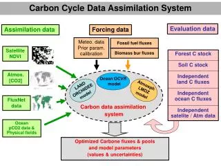
Carbon Cycle Data Assimilation System (CCDAS) Assimilated Prescribed Assimilated CO2 + Uncert. veg. index satellite + Uncert. Phenology Hydrology CCDAS Step 2 BETHY+TM2 only Photosynthesis, Energy&Carbon Balance CCDAS Step 1 full BETHY Background CO2 fluxes* Optimized Params + Uncert. Diagnostics + Uncert. * * ocean: Takahashi et al. (1999), LeQuere et al. (2000); emissions: Marland et al. (2001), Andres et al. (1996); land use: Houghton et al. (1990)
BETHY(Biosphere Energy-Transfer-Hydrology Scheme) lat, lon = 2 deg • GPP: C3 photosynthesis – Farquhar et al. (1980) C4 photosynthesis – Collatz et al. (1992) stomata – Knorr (1997) • Raut: maintenance respiration = f(Nleaf, T) – Farquhar, Ryan (1991) growth respiration ~ NPP – Ryan (1991) • Rhet: fast/slow pool resp. = wkQ10 T/10 C fast/slow / t fast/slow • slow –> infin. average NPP = b average Rhet (at each grid point) t=1h t=1h t=1day b<1: source b>1: sink
Major El Niño events Major La Niña event Post Pinatubo Period global fluxes Optimised fluxes (1)
correlation between Niño-3 SST anomaly and net CO2 flux shows maximum at 4 months lag, for both El Niño and La Niña states lag correlation (low-pass filtered) Optimised fluxes (2) normalized CO2 flux and ENSO ENSO and terr. biosph. CO2: correlation seems strong
flux sites? net CO2 flux to atm. gC / (m2 month) during El Niño (>+1s) lagged correlation at 99% significance -0.8 -0.4 0 0.4 0.8 Optimised fluxes (3)
Second Derivative (Hessian) of J(m): ∂2J(m)/∂m2 yields curvature of J, provides estimated uncertainty in mopt J(x) Space of m (model parameters) Error Covariances in Parameters Figure taken from Tarantola '87
examples: measurements model diagnostics error covariance matrix of measurements Error covariance of parameters after optimisation: = inverse Hessian Error Covariances in Parameters Cost function (misift): assumed model parameters a priori covariance matrix of parameter + model error a priori parameter values
Error Covariances in Diagnostics Error covariance of diagnostics, y, after optimisation (e.g. CO2 fluxes): adjoint or tangent linear model error covariance of parameters
a priori mean/uncertainties a posteriori mean/uncertainties Comparison shows impact of a (pseudo) flux measurement in the broadleaf evergreen biome on Q10 estimated by an inversion of SDBM: Upper panel: only concentration data Lower panel: concentration data + pseudo flux measurement (mean: as predicted sigma: 10gC/m^2/year) Details: Kaminski et al., GBC, 2001
Conclusions • CCDAS with 58 parameters can already fit 20 years of CO2 concentration data • Sizeable reduction of uncertainty for ~13 parameters • terr. biosphere response to climate fluctuations dominated by ENSO • System can test model with uncertain parameters, and deliver a posteriori uncertainties on parameters, fluxes
Outlook • explore more parameter configurations • include fire as a process with uncertainties • need more constraints, e.g. eddy fluxes –> reduce uncertainties • however: needs to solve scaling problem (satellites?) • approach can be regionalized easily • extend approach to ocean carbon cycle • projection of uncertainties into future