Download
1 / 30
300 likes | 535 Views
The EC-Carbon Assimilation System. Saroja Polavarapu, Ray Nassar, Doug Chan (CCMR/CRD) Dylan Jones, Mike Neish, Shuzhan Ren, Feng Deng (U Toronto) John Lin, Myung Kim (U Waterloo). Meeting on Air Quality Data Assimilation and Fusion R&D, Jan. 16-17, 2011. Pg C/yr. 8.6.

E N D
The EC-Carbon Assimilation System Saroja Polavarapu, Ray Nassar, Doug Chan (CCMR/CRD) Dylan Jones, Mike Neish, Shuzhan Ren, Feng Deng (U Toronto) John Lin, Myung Kim (U Waterloo) Meeting on Air Quality Data Assimilation and Fusion R&D, Jan. 16-17, 2011
Pg C/yr 8.6 The Global Carbon Cycle • The natural carbon cycle involves CO2 exchange between the terrestrial biosphere, oceans/lakes and the atmosphere. • Fossil fuel combustion and anthropogenic land use are additional sources of CO2 to the atmosphere. http://www.scidacreview.org/0703/html/biopilot.html
The Global Carbon Cycle [IPCC, 2007] • Only 50-60% of anthropogenic CO2 emissions remain in the atmosphere • The uncertainty and interannual variability in the global CO2 uptake is mainly attributed to the terrestrial biosphere • Reducing uncertainties in CO2 sources and sinks is an active area of research and has important implications for climate mitigation policies.
Greenhouse gas measurement network NOAA-ESRL (US), Environment Canada, CSIRO (Australia), JMA (Japan) ... WMO - World Data Centre for Greenhouse Gases (WDCGG) • Numerous research groups over the past ~20 years have combined the highly-accurate but sparse atmospheric CO2 measurements from the ground-based network with models, to give estimates of CO2 sources and sinks on coarse spatial scales. • With the coming wealth of satellite observations, more sophisticated methods of data assimilation that can handle the large data volume needed to provide estimates on finer scales. http://gaw.kishou.go.jp/cgi-bin/wdcgg/map_search.cgi
Variations in Atmospheric CO2 Modeled CO2 at Park Falls • Diurnal variations, linked to surface sources and sinks, are strongly attenuated in the free troposphere • Diurnal variations in column CO2 are less than 1 ppm • Large changes in the column reflect the accumulated influence of the surface sources and sinks on timescales of several days Column CO2 Surface CO2 Diurnally varying surface fluxes 5-day running mean surface fluxes [Olsen and Randerson, JGR, 2004]
Satellite observations • Surface observations are highly accurate but sparse • Satellite observations can complement spatial coverage though vertical resolution of nadir obs is typically poor • Current missions (nadir): HIRS (1978-), AIRS (2002+), SCIAMACHY (2003+), TES (2006+), IASI (2007+), GOSAT (2009+) • Current missions (limb): ACE-FTS (2004+) • Future missions: IASI (2012,2016), OCO-2 (2013/4), TanSat (2015), GOSAT-2 (2016), CarbonSat (2018), PCW/PHEMOS-FTS (2018), ASCENDS (2020)
Strategies for Temporal and Spatial Coverage Slide from Ray Nassar, CCMR • Sun-synchronous Low Earth Orbit (LEO) missions only measure at a single point in the diurnal cycle • Increasing temporal coverage requires a constellation of LEO satellites or different orbits • CarbonSat constellation of 3 - 5 LEO satellites has been proposed • Geostationary missions like NASA’s GEO-CAPE could have CO2 capability added for continuous coverage from ~50°S-50°N • Canada’s Polar Communications and Weather (PCW) Polar Highly Elliptical Molniya Orbit Science (PHEMOS) Weather, Climate and Air quality (WCA) proposal (currently in phase-A) would use a Highly Elliptical Orbit (HEO) for high latitude quasi-continuous coverage
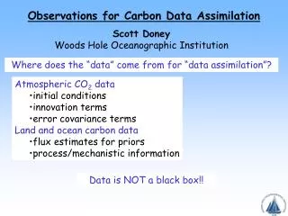
Estimating CO2 fluxes from surface • Can use all observations over a time window to estimate CO2 fluxes at all times • Standard method is Bayesian Synthesis Inversion • EC CO2 flux inversion capability: • Bayesian Synthesis Inversion • Transport model: NIES (Japan), TM5 (Europe), GEOS-Chem (US) • Ground-based observations • Can standard methods of flux estimation handle coming wealth of observations? dCO2/dt = transport + flux photo credit: Matt Rogers, Colorado State University
previous estimate Connection between obs and fluxes at all previous times for all regions. 264 model integrations of 1 year All source region amplitudes at all times ~22x12=264 All observations at all times ~100x12=1200 The flux estimation problem Estimate monthly averaged fluxes from ground-based obs for 1 year As number of source regions increases too many model integrations!
Bayesian Synthesis Inversions Advantages: • Uses all obs at all times (months) to determine all monthly fluxes over 1-3 years • If assumptions are correct, this is the best, most general solution Problem 1: • Want to use more obs (e.g. continuous, aircraft, satellite) so we can capture finer time and space scales in fluxes • Solution 1: Use 4D-Var (e.g. GEOS-Chem, Chevallier et al. (2007,9)) • ~100 forward+ADJ runs • Need to develop and maintain TLM and ADJ models • Solution 2: Use Kalman smoother (e.g CarbonTracker) • Sequential estimation means using obs only over a short time period, then marching forward. Smoother means improving estimate based on future obs • Does not use all obs to estimate all sources
The flux estimation problem Estimate monthly averaged fluxes from ground-based obs for 1 year • Random errors due to: • Initial conditions in CO2 • Driving wind analyses • Model formulation • representativeness • Instrument error • 1200x1200 Random errors in source amplitudes 264x264 All error sources convolved into 1 error estimate (R). In practice only obs and rep errors are accounted for. Often, no correlations are assumed.
If B and R are incorrect, then uncertainty estimates are wrong The flux estimation problem Estimate monthly averaged fluxes from ground-based obs for 1 year • Random errors due to: • Initial conditions in CO2 • Driving wind analyses • Model formulation • representativeness • Instrument error • 1200x1200 Random errors in source amplitudes 264x264 Estimation error
Relaxing the assumptions Problem 2: Assumptions made in practice are not correct, • e.g. no errors for analysed wind fields, initial CO2 field, model formulation, source region definitions. Often no error correlations. • Because assumptions are not valid, we cannot believe uncertainties Solution: Use data assimilation to estimate concentrations, simultaneously inferring fluxes as a “model parameter or forcing” • Use ensemble of forecasts to explicitly account for initial state, meteorology, model, representativeness, obs, source region errors. • Fully evolve covariances in time, producing full spatial correlations • Ensemble Kalman Smoother used by Japanese (Miyazaki 2011, JGR) for CO2 fluxes.
Analysis step forecast step EC-CAS Carbon Assimilation System Flask, continuous, aircraft, satellite Perturb initial conc., met fields, fluxes Perturb obs
EC-CAS: Carbon Assimilation System • New EC-CAS (Carbon Assimilation System) proposed for monitoring carbon and policy/verification purposes • Project started in April 2011. EC/UT/UW collaboration. • Can be used to answer questions on observing system needs (space-based, and EC’s ground-based obs) • Will be run routinely but behind real time since it takes time for flux to reach measurement locations. • EC-CAS is based on EnsKF with GEM-MACH but will be a Kalman smoother for estimating surface fluxes • Parameters for EnsKF not clear yet: update frequency, and data window (6h normally)
The future vision: Comprehensive Carbon Data Assimilation System • EC-CAS will form the basis of a comprehensive carbon assimilation system, comparable to those of NASA, NOAA and agency-consortiums in Europe and Japan.
D.Chan/M.Ishizawa had CO2 version with GEM v3.2.0 to see if GEM can capture synoptic scale variability. It does seem to do this The minimum CO2 concentration during these two months was subtracted so the time series start from a zero value. Complete time series (top) Daily variability was removed by plotting afternoon mean values only (bottom) Starting point with GEM Figure from D. Chan, CCMR Time series of CO2 at Fraserdale
Early issues with model choice • Our development uses MAESTRO which is used to run the EnsKF (CMC uses this for operational EPS) • Choice of GEM version for EC-CAS: • EnsKF uses GEM v4.2.0 and is not backward compatible so Doug Chan’s GEM v3.2.0 with CO2 tracer v3.2.0 not feasible. • Decided to choose GEM-MACH because it already handles emissions, tracers, vertical diffusion and they will move to v4.4.0. Also this permits future interaction and collaboration with AQRD. • Model testing with GEM-MACH (v3.3.3) but EnsKF development needs v4.4.0 which is under beta testing.
GEM-MACH-GHG version • GEM-MACH was developed for CO2 simulation by • Started from global version (based on v3.3.3) used for stratospheric ozone and developed by Jean deGrandpre (ARQI) • Reduced resolution to 400x200 (roughly 1 degree), 80 levels • Adding 6 CO2 tracers, one for each emission source plus a total CO2 and a background CO2 (with no emissions) • Coupled tracers to emissions fields • Obtained monthly emissions from Doug Chan, and regridded these to Z grid, 400x200 (preserving total mass) • Uses GEM-MACH emissions preprocessor with global fields
Model validation run • How well can GEM-MACH simulate Carbon? Key concern: mass conservation over multiyear runs. Diagnostics: Seasonal cycle, hemispheric gradients, mass conservation. Comparison against obs and other models (CarbonTracker, GEOS-Chem) • Simulation for January 1, 2009 – Jan. 2012? • Dates related to GOSAT launch (Jan. 2009) and GEM-strato analyses availability (Operational implementation on June 22, 2009) • Initial condition from CarbonTracker for Jan. 1, 2009 • Meteorology: surface fields (archived surface analyses), 3D winds (prelim cycle, parallel run, operations) • Emissions: • Every 3 hours (area type) though GEM-MACH set up for monthly fields with diurnal variation • biosphere (CarbonTracker a posteriori) • ocean (CarbonTracker a posteriori) • Fossil Fuel (CDIAC) • Biomass burning (GFED v3)
EC-CAS development priorities • Model • GEM-MACH based on v4.4.0 beta-9 runs in CO2 mode w/o emissions. Need to add emissions. Reconnect vertical diffusion. • Repeat model validation run with GEM-MACH-GHG v4.4.0 • Assimilation (EnsKF) • Allow EnsKF and MAESTRO to use GEM-MACH instead of GEM • Change control vector change from meteorology to tracers/species + fluxes • Develop observation operators for all new obs to be assimilated or monitored • Complete EnsKF and test with surface obs • Extend EnsKF to a Kalman Smoother (use future obs to estimate current flux) • Observations • convert surface obs to BURP for ingestion by data assimilation codes. • examine GOSAT data, determine biases, quality control procedures, bias correction procedures. • Emissions • Incorporate diurnal/weekly scaling factors developed by Ray Nassar
GHG and AQ assimilation synergies • GEM-MACH development can be coordinated, e.g. vertical diffusion, mass conservation • EnsKF development by EC-CAS will be usable (but not tested) with reactive chemistry
Observations from a Three-Apogee Orbit Slide from Ray Nassar, CCMR 2 satellites, each with 16 h orbit apogee = 43 500 km perigee = 8100 km Images 16 h / 48 h per region 8 (60x60) arrays wide 6 (60x60) arrays tall 10 x 10 km2 footprint NIR-TIR FTS similar to GOSAT TANSO-FTS (ABB Group) could measure CO2 and CH4 over ice-free land surfaces Nassar et al. (in prep.) Various pointing scenarios for PCW-PHEMOS are currently under consideration
Canadian Greenhouse Gas Measurement Program Figure from Elton Chan
Global Greenhouse Gas Measurement Network World Data Centre for Greenhouse Gases NOAA-ESRL (US), Environment Canada, CSIRO (Australia), JMA (Japan) ... WMO - World Data Centre for Greenhouse Gases (WDCGG)
Present satellite instruments All are nadir except ACE which is occultation (limb)
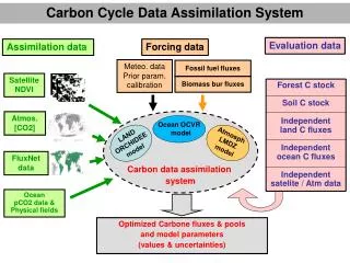
CO2 Flux Inversion with Regional Focus on North America Deng et al. (2007) 30 small regions in North America, 20 large regions for the rest of the globe, and 88 CO2 stations (GlobalView-2005)
Annual Result for 2003 Deng et al. (2007) North American biosphere is a sink of −0.97 ± 0.21 Pg C, Canada’s sink is −0.34 ± 0.14 Pg C.