Download
1 / 46
460 likes | 587 Views
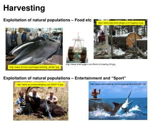
http://www.cairnsfishing.com/images/photos/photo61.jpg. Exploitation of natural populations – Food etc. http://www.lakeviewcottage.com/logging-2.jpg. http://www.accuratereloading.com/z200110.jpg. Exploitation of natural populations – Entertainment and “Sport”.

E N D
http://www.cairnsfishing.com/images/photos/photo61.jpg Exploitation of natural populations – Food etc http://www.lakeviewcottage.com/logging-2.jpg http://www.accuratereloading.com/z200110.jpg Exploitation of natural populations – Entertainment and “Sport” http://www.mmcta.org/images/whaling_whale1.jpg http://www.treehugger.com/files/nz-trawling-02.jpg Harvesting
Agriculture http://www.ext.vt.edu/pubs/forestry/446-603/pine.jpg Management (?) http://www.prijatelji-zivotinja.hr/data/image_1_419.jpg http://www.kaingo.com/images/footer/quelea.jpg
http://io.uwinnipeg.ca/~simmons/images/lb7fg1a.gif http://www.bu.edu/lernet/GK12/eric/earthworm.jpg t0, N0 = 7 t1, N1 = 9 t2, N2 = 11 t3, N3 = 13 SUSTAINABILITY Imagine an earthworm* – 7 segments long This earthworm produces two segments per day * - Dr Anesh Govendar’s “Earth-worm model”
7 + 2 = 9 9 – 3 = 6 t0, N0 = 7 t2, N2 = 5 t1, N1 = 6 t3, N3 = 4 t4, N4 = 3 t5, N5 = 2 Over-exploitation What is the maximum sustainable number of segments that can be harvested each day? If you harvest three segments per day:
Under-exploitation 7 + 2 = 9 9 – 1 = 8 t1, N1 = 8 t0, N0 = 7 t2, N2 = 9 t3, N3 = 10 t4, N4 = 11 t5, N5 = 12 If you harvest one segment per day:
7 + 2 = 9 9 – 2 = 7 t0, N0 = 7 t1, N1 = 7 t2, N2 = 7 t3, N3 = 7 t4, N4 = 7 t5, N5 = 7 t6, N6 = 7 If you harvest two segments per day:
Population Size Not Sustainable Sustainable Maximum Harvest Total over 12 day projection: 3 per day = 15 1 per day = 12 2 per day = 24
Building harvesting into a model Model applies for a species showing discrete breeding – use R not r Assume intra-specific competition occurs Nt+1 = (Nt R) / {1 + [Nt.(R-1)/K]} Step 1 Project population into future for x time units without competition Calculate R and recruitment (additions) for each time step Plot population size against time (line-graph) Plot recruitment against population size (X-Y graph) Determine what the maximum recruitment is and when it occurs
Project 100 years If N0 = 12, R = 1.63, K = 368 974
Step 2 We will start by using a constant yield model (i.e. a fixed number of individuals are harvested from the population each year) Label a cell Fixed Annual Yield and, in the adjacent cell, put an arbitrary starting value – say 1 Create a harvest (h) column next to the “additions” column. This is the number of individuals that you are going to harvest in each interval. Make each cell address equal to the value of your Fixed Annual Yield, with the exception of t0, which make equal to 0 Calculate Total harvest over the 100-year projection by summing the harvest column (should equal 100, at this stage) You must now subtract the harvest each year from the numbers in the population …….BUT…….do you subtract the harvest from the population BEFORE or AFTER it has reproduced? What is the difference? Constant Yield Model Nt+1 = ((Nt – ht+1).R) / {1 + [(Nt – ht+1).(R-1)/K]} Nt+1 = ((Nt R) / {1 + [Nt.(R-1)/K]}) – ht+1
AFTER BEFORE
STEP 3 Adjust your value of Fixed Annual Yield and adjust the time of first harvesting in order to maximise the total harvest over the 100 year projection BUT remember – it is important that the final R (R99) value is greater than or equal to 1.0000 (i.e. the population is sustainable) PLAY Advantages Fixed Yield Models are liked by industry because they can plan plant and workforce in advance Communities like Fixed Yield Models because they know how much money will be coming in – in advance Disadvantages Data-hungry: small errors in Yield can result in population crashes
Management implications of MSY models • Set a Total Allowable Catch (TAC) each year • Apportion TAC amongst rights’ holders • Open the resource to exploitation • Keep a cumulative log of harvest and close access to right’s holder when TAC reached
Look at the Stock : Recruit curve Maximum recruitment to the population occurs not at the carrying capacity (when the population size is at its maximum), but at some intermediate density. If you allow the population to increase beyond this intermediate density you are decrease the number of recruits. How do you calculate MSY without playing around? Remember the earthworm model – the MSY was achieved by harvesting the number of “recruiting” segments to the worm (population): two per day. How do we find the equivalent of the “two segments per day” MSY in our population?
How do we know when to start harvesting? Look at the relationship between recruitment and time. In this case we should start harvesting 44 524 individuals from time 22 In our example here – the maximum number of individuals that recruit to the population is 44 524 over the period 21- 22
If you remove this number of individuals (starting at time 22), the population will remain at a constant size. In other words these individuals are surplus to the population and we refer to this type of model as a Surplus Production Model.
Garbage OVER - Exploitation UNDER - Exploitation MSY - 10% MSY + 10% Small errors in MSY can have BIG consequences
http://www.pmel.noaa.gov/foci/sebscc/results/megrey/spawner-recruit.gifhttp://www.pmel.noaa.gov/foci/sebscc/results/megrey/spawner-recruit.gif http://oregonstate.edu/instruct/fw465/sampson/anchovy/anchov18.jpg Walleye-Pollock E Beiring Sea Anchovetta Peru http://www.fao.org/docrep/W5449E/w5449ekz.gif http://fwcb.cfans.umn.edu/courses/FW5601/ALAB/lab10/SRResources/image27.gif Some Stock Recruit Curves
Harvesting from a population (in a sustainable way) does not harm the population. WHY? By preventing a population from reaching the carrying capacity, you maintain it in a constant state of growth and ensure that the negative effects of intra-specific competition are reduced.
Constant Effort Model Let us imagine a population, size N. You go out today and spend 2 hours harvesting from the population (with efficiency e) and come back with aa individuals But you went out yesterday and spent 4 hours harvesting from the population (with efficiency e), and came back with bb individuals Which is larger: aa or bb? WHY?
http://www.jenskleemann.de/wissen/bildung/media/6/65/fishing_trawler.jpghttp://www.jenskleemann.de/wissen/bildung/media/6/65/fishing_trawler.jpg Let us imagine a fish population, size N. You go out today and spend 2 hours harvesting from the population using a motor-powered vessel and a trawl net and come back with aa individuals But you went out yesterday and spent 2 hours harvesting from the population using a canoe and a throw net, and came back with bb individuals Which is larger: aa or bb? WHY? http://www.hope-for-children.org/images/transafrica_moz03.jpg
NOW – You go out today and spend 2 hours harvesting from the population using a motor-powered vessel and a net and come back with 120 546 individuals But you went out yesterday and spent 2 hours harvesting from the population using a motor-powered vessel and a net and came back with 98 113 individuals WHY?
Catch is proportional to effort, efficiency and population size. If we fix efficiency (assume hereafter that it is equal to 1), then catch will reflect population size and effort. If we fix effort, then catch will reflect population size: in other words the numbers caught will reflect some fixed proportion of the population.
Building a Constant Effort Model Step 2 Label a cell Efficiency and, in the adjacent cell, enter a value of 1 (100% efficient) Label a cell Effort and, in the adjacent cell, put an arbitrary starting value – say 0.1. You are going to play around with this number in just a minute. Label a cell EE (Effort x Efficiency) and make it equal to the product of the aforementioned Efficiency and Effort cells (it should equal 0.1). Create a harvest (h) column next to the “additions” column. This is the number of individuals that you are going to harvest in each interval. Make this number in each cell equal to the product of the EE cell and the population size: with the exception of t0, which make equal to 0 In order to avoid circular arguments that will arise when you subtract the harvest from the population size, you need to re-enter the formula to calculate population size at t+1 into the harvest calculations. Thus – the harvest at (e.g.) t5 is calculated as h5 = ((N4 R) / {1 + [N4.(R-1)/K]}) * EE
Step 2 Calculate Total harvest over the 100-year projection by summing the harvest column You must now subtract the harvest each year from the numbers in the population …….BUT…….do you subtract the harvest from the population BEFORE or AFTER it has reproduced? What is the difference? Nt+1 = ((Nt – ht+1).R) / {1 + [(Nt – ht+1).(R-1)/K]} Nt+1 = ((Nt R) / {1 + [Nt.(R-1)/K]}) – ht+1
Harvesting after reproduction The shape of both lines should be similar – one is just 10% of the other (EE = 0.1) Total Harvest = 2 258 460
Harvesting BEFORE or AFTER the population has had a chance to reproduce can have profound impacts on population size! AFTER BEFORE
STEP 3 Adjust your value of EFFORT and adjust the time of first harvesting in order to maximise the total harvest over the 100 year projection BUT remember – it is important that the final R (R99) value is greater than or equal to 1.0000 (i.e. the population is sustainable) PLAY Advantages Fixed Effort Models are liked by management authorities because they are not as sensitive as Fixed Yield models to mistakes. A 10% change in effort will not necessarily crash the population, whilst a 10% increase in a Fixed Yield probably will! Disadvantages Because the numbers harvested each year will vary (with population size), industry and communities have problems planning in advance.
Management implications of MSY models • Set a Total Effort each year • Apportion Effort amongst rights’ holders • Open the resource to exploitation • Keep a cumulative log of effort and close access to rights’ holder when Total Effort reached • Effort can be limited by (in the case of fishing) • Closed seasons • Closed areas • Fleet size, vessel type, engine power • Gear used: number of hooks or lines, mesh size of nets • Time at sea • etc
Building environmental variability into your models All the models you have developed so far are deterministic (essentially fixed), but we know that populations change in size all the time due to extrinsic factors such as the weather. Weather conditions have an impact on the amount of resources available to a population, which in turn influences the carrying capacity. We need to build some sort of environmental variability into our models if they are to more “accurately” reflect patterns in the real world, and to minimise the chance of over-exploiting the population when we start to harvest. Before we start this exercise, we need to know how often “bad” or “good” weather conditions occur, and we need to know how these affect the carrying capacity. Whilst the first set of information can be readily obtained from long-term weather sets, the latter is difficult to pin down. That does not matter in a modeling scenario – because we are exploring the processes rather than the actual numbers. In our models, we are going to use random numbers to indicate the state of the weather each year, and we are going to ask MSExcel to look at these numbers and see if they are greater or less than the numbers we propose to indicate “good” or “bad” weather, and then to assign a carrying capacity accordingly. This modified k value will then be used in our equations to model population size
http://www.lewes-flood-action.org.uk/lfa-images/spenceslane.jpghttp://www.lewes-flood-action.org.uk/lfa-images/spenceslane.jpg http://i1.trekearth.com/photos/16779/drought-victim.jpg http://www.cmhenderson.com/images/jsrnclds.jpg Weather calculations If “bad” weather happens, on average, once every 15 years, we can say that the probability of bad weather is 1 / 15 = 0.0667 If “good” weather happens, on average, once every 9 years, we can say that the probability of good weather is 1 / 9 = 0.111
Incorporating weather into an unexploited population with: N0 = 12, R = 1.63, K = 368 974 In your spreadsheet, you should set up a new column labeled “Weather A”. Weather is a random number in our model, so ask MSExcel to generate a random number each year =RAND() At this point, no two of us are going to have the same weather conditions. Every time you do something to the worksheet, your weather conditions will change (as they will too if you press the F9 key). You can convert the constantly changing numbers into values using the edit, copy, paste special, values function – BUT DON’T yet The next thing we need to do is to ask MSExcel to identify the weather each year as Good, Bad or Normal, and we do this using the IF function. The logic of the IF function is as follows…. We ask MSExcel to look at the contents of a particular cell address and if the contents conform to some pre-established condition, then it will return one answer and if it doesn’t then it will return another answer
For example – Set up a dataset spanning four columns (A-D) and 10 rows. Put titles to each column in row 1 as indicated, and fill column A with random numbers. In column B, we are going to ask MSExcel to look at each cell in column A and, if it is smaller than 0.20, to return a value of “YES” in the corresponding cell of Column B. Otherwise to return a value of “NO” The “ ” signs are important when dealing with text in formulae, but should be ignored if using numbers =IF(A2<0.20,”YES”,”NO”) Repeat the exercise for column c You can combine IF arguments. For example, in column D we are asking MSExcel to look at the contents of cells in column A and then IF they are larger than 0.9 to assign an answer of “BIG”, IF they are smaller than 0.2 to assign an answer of “SMALL”, otherwise to return an answer of “Average” =IF(A2<0.20,”SMALL”,IF(A2>0.90,”BIG”,”Average”))
Okay – having set up our weather (in Weather A), define it as GOOD, BAD or NORMAL in a Weather B column using the =IF Function
Weather is a random number in our model and varies from 0.0000 – 1.0000 The probability of bad weather is 0.0667: the probability of good weather is 0.111 In other words, if the random number is less than 0.0667, then it must be bad weather 0.0667 0.1111 Bad Weather Good Weather On the other hand, if the random number is more than 0.8889 (1.0000 – 0.1111) , then it must be good weather 1.0000 Random Number How?
1 2 3 4 5 6 7 8 9 Next you must set new K values based upon the effect that weather has on K Under Good weather conditions New K = 1.69K Under Bad weather conditions, New K = 0.25K Under Normal weather conditions New K = K A B C D E F G Use another =IF function =IF(F9=“GOOD”,G$6,IF(F9=“BAD”,G$4,B$2))
You must now make your population numbers reflect this new K value REMEMBER – NO TWO will have the same results
Okay – having now built weather into your model for an unexploited population – you must now build it into your Fixed Yield and Fixed Effort harvesting models Remember – the population must not crash in your simulations, the Final R (R99) should be greater than or equal to 1.0000, and you should aim to maximize the harvest over the 100 year period PLAY Your model run is from a single simulation – based on the particular set of random numbers generated in that single run. Ideally you need to repeat the simulation (looking at final R, total harvest, and whether the population crashes or not) thousands of times for each starting time, fixed yield and fixed effort model that you use in order to come up with appropriate values! You can do this using macros………………but that is another story!
R = 1.63 The age structured models we have constructed ignore intra-specific competition and are based on a constant R – i.e. exponential models The models built to date assume that all individuals in the population are equal Age Structured Harvesting We know that this is not reasonable How can we build harvesting into an age-specific model? Not easily…………………..certainly not in this course
That said – when you start to harvest from a population (inevitably during its growth phase), the population is maintained in a constant state of growth Population (growing under intra-specific competition) Harvest (MSY) Population (growing without intra-specific competition) As a consequence, using Fixed R Models may not be unreasonable……….
So………………… Start off with the basic life table, calculate p and m, and project the population into the future (e.g.) 100 time units. Plot total population size against time Calculate Reproductive Value
Subtract harvest from the population table: BEFORE OR AFTER REPRODUCTION? Set up a parallel table with harvest information – i.e. the number of individuals of each age class you will harvest each year Use a fixed yield model – i.e. harvest a fixed number (h) of individuals of each age class at each time interval and make each value in the harvest column for a particular age class equal to the h value for that age class at t0, all h values = 0: harvest 1 0 year old from t1: keep a running total
PLAY Adjust harvest of each age class, adjust time of first harvest in order to maximize total harvest. REMEMBER – Population must not crash!
Optimising harvest in an age-structured model can be time-consuming! Better yields were (in any case) obtained from harvesting under a constant effort scenario in our previous models and there is no reason to suppose that this will be different here! It is also quicker!!! Start off as before with a population table and a parallel harvest table. Set the harvest table up with an Effort row, an Efficiency row and an EE row (Effort x Efficiency). All values in the Efficiency row should equal 1 (i.e. the harvesting method is 100% efficient). In the first instance make all values of Effort = 0, except E0 (=0.00000001). That means all values of EE will equal 0, except EE0, which will equal 0.00000001
You now need to make the harvest of a particular age class at a particular time equal to EE multiplied by the number of individuals of that age class at that time. Having done that, you will need to subtract this number from the number of individuals of that age at that time from the population table. This will inevitably result in Circular Argument errors in MSExcel….which means that you need to build the formulae projecting populations into the future into the harvest table too! Ensure that harvest at t0 = 0 With such a low level of Effort, you should only start to harvest any whole organisms at time 32
Adjust Effort of each age class, adjust time of first harvest in order to maximize total harvest. REMEMBER – Population must not crash! PLAY