Download
1 / 51
510 likes | 640 Views
US GLOBEC Meeting Boulder, Colorado Feb. 17, 2009. Results From Comparative Ecosystem Studies within GLOBEC: Examples from SPACC, CCC and ESSAS. Ken Drinkwater Institute of Marine Research and Bjerknes Center for Climate Research, Bergen, Norway. Outline. Why comparative studies?

E N D
US GLOBEC Meeting Boulder, Colorado Feb. 17, 2009 Results From Comparative Ecosystem Studies within GLOBEC: Examples from SPACC, CCC and ESSAS Ken Drinkwater Institute of Marine Research and Bjerknes Center for Climate Research, Bergen, Norway
Outline • Why comparative studies? • Types of comparisons • Examples • Species –Cod, Lobster • Ecosystems – Upwelling, Subarctic Seas • Problems • Concluding Remarks
Why Comparative Studies of Ecosystems? • Cannot run controlled experiments on ecosystems 2. Provides insights that one cannot obtain by looking at a single ecosystem 3. Ecosystems are complex – can help determine what is a fundamental process and what is unique. 4. Increases statistical degrees of freedom 5. Sharing approaches and methodologies
Types of Comparisons There are many types of comparative studies. 1. Same ecosystem type but different geographic regions (upwelling regions, subarctic seas) 2. Different ecosystems, e.g. tropics vs. polar ecosystems. 3. Same species but different geographic (hydrographic) regions, e.g. Atlantic cod, American lobster. 4. Same ecosystem (geographic area) but at different times (forcing), e.g. cold period vs. warm period.
Atlantic Cod (Gadus morhua) CCC (Cod and Climate Change)
Temperature plays a large role in determining the Growth Rate of cod The relative size of a 4-year old as a function of mean bottom temperature. Brander1994
The same information shown graphically, i.e. the relative size of the age 4 cod at different temperatures.
Cod Recruitment and Temperature Faroes 4 Warm Temperatures decrease Recruitment Warm Temperatures increase Recruitment 2 0 -2 -2 -1 0 1 2 Georges Bank 4 Iceland 4 7 2 2 0 0 -2 -2 -2 -1 0 1 2 -2 -1 0 1 2 4 4 North Sea Barents Sea 6 8 2 2 0 0 -2 -2 -2 -1 0 1 2 - -2 -1 0 1 4 4 W. Greenland 4 Irish Sea 4 9 Log2 Recruitment Anomaly 2 2 0 0 -2 -2 -2 -1 0 1 2 4 -2 -1 0 1 2 Newfoundland 10 Celtic Sea 2 3 4 Temperature Anomaly 0 2 -2 0 Mean Annual Bottom Temperature -2 -2 -1 0 1 2 -2 -1 0 1 2 2 11
Lobster Landings Magdalen Island In the late 1980s landings rose dramatically with suggestions that it was due to good management.
Again a dramatic rise in landings in the late 1980s-early 1990s and claims that management was working well.
US and Canadian Lobster Landings The US and Canadian landings for each of the lobster management regions showed similar trends (except for 4 out of 34) with different management strategies. Could not have been management strategies. It was not increased effort.
SPACC (Small Pelagics and Climate Change)
Synchrony in Upwelling Areas Kawasaki, 1983; Bakun, 1997 Bakun, 1989; 1997 Lead to much research on ecological teleconnections.
Also found tendency for anchovy and sardines to be out of phase (but not always or everywhere). Lluch-Belda et al., 1989
ESSAS (Ecosystem Studies of Sub-Arctic Seas)
NORCAN (Norway-Canada Comparison of Marine Ecosystems) SSTs in the Labrador Sea Coccolithophore Bloom at the eastern entrance to the Barents Sea
NORCAN • WorkshopFunded by NRC and DFO • Held in Bergen in December 2005 • Meeting in St. John’s May 2006 and writinggroups met in Bergen 2007 • Decided to writepapersalongdiscipline lines – physicaloceanography, phytoplankton, zooplankton, fish (3) and marine mammals. • Drafts nearingcompletion and hope to submit mid-2009
KOLA SEAL ISLAND BONAVISTA • Ocean Temperature Trends between two regions Out-Of-Phase prior to mid-1990s • Similar Trends Recently
Normalized indices (blue-cold, fresh; red-warm, saline) used to estimate overall index for both Labrador and Norwegian regions.
These standardized anomalies also show change from out of phase prior to the mid-1990s and in phase since then.
MEAN ANOMALY 1991 2000 2003 NORTH ATLANTIC WINTER SLP FIELDS HISTORICAL PATTERN- COLD IN WEST WARM IN EAST EASTWARD DISPLACEMENT WESTWARD DISPLACEMENT
NOAA Fisheries MENU (Marine Ecosystem Comparisons of Norway and the United States)
MENU • WorkshopFunded by NRC • Held outside Bergen in March 2007 • Brought data to thetable • Dividedinto 2 groups: (1) response to recentchanges and (2) structure and functionofecosystem. • Five papers have beenaccepted for publication in PiO.
Russia Menu Regions Greenland Alaska Barents Sea Eastern Bering Sea (EBS) (NOR/BAR) Norwegian Sea Gulf of Alaska (GOA) AreaLatitude Canada GOM GB USA Gulf of Maine / Georges Bank (GOM/GB)
MeanCirculation Strong Tidal Currents and Mixing in subregions Highly Advective Systems
Correlations between annual heat fluxes and SST temperatures Pacific Ecosystems: Significant correlations, 25-30% of SST variance accounted for. Atlantic Ecosystems: Weak and non-significant correlations. Suggests that warming due to advection in the Atlantic while in Pacific air-sea fluxes play a significant role.
Gulf of Alaska Salinity In GoA surface freshening due to local runoff In GoM freshening due to advection from the North (Arctic?) Gulf of Maine Barents Sea In Barents Sea increasing salinity due to higher salinity in Atlantic Water.
SeaWiFS climatology – Chl. a (Apr-Jun) Norwegian Sea / Barents Sea Bering Sea / Gulf of Alaska Gulf of Maine / Georges Bank Mueter et al., in press Source: http://oceancolor.gsfc.nasa.gov/cgi/level3.pl
Productivity increases with nitrate content of deep source waters Approximate range Nitrate in source waters and total annual primary production GOM/GB Mueter et al., in press
Effect of SST on primary production, 1998-2006 Gulf of Maine/ Georges Bank 500 (P < 0.001) Gulf of Alaska 400 Total annual net primary production (gC m-2) (n.s.) Bering Sea (P = 0.039) 300 200 Norwegian Sea Barents Sea (n.s.) (P = 0.093) 2 4 6 8 10 Mueter et al., in press Annual mean SST (°C)
NOAA Fisheries MENUII
MENUII • With thesuccessof MENU, NOAA and IMR administrators encouraged MENU participants to submit full proposals • Decidedthatemphasiswould be modelcomparisons and ecosystemindicators • 4 types ofmodels: ECOPATH, productionmodels, biophysicalmodels (3-D hydrodynamicmodels up to zooplankton) and system models (includesfish and fisheries (ATLANTIS)
ATLANTIS Ecosystems are created in Atlantis three-dimensionally, using linked polygons that represent major geographical features. Information is added on local oceanography, chemistry and biology such as currents, nutrients, plankton, invertebrates and fish. The model then simulates ecological processes such as: consumption and production, waste production, migration, Predation, habitat dependency, mortality. The Atlantis framework used for management strategy evaluation incorporates a range of sub-models for each major step in the management cycle. They simulate the marine environment, the behaviour of industry, fishery monitoring and assessment processes, and management actions and implementation.
MENUII • Same modeldifferent regions • Differentmodels for same region • Determinewhatwelearned from eachofthemodels A good forecaster (modeller) is not smarter than everyone else, he merely has his ignorance better organised. -Anonymous
MENUII • Norwegian component funded by RCN (2009-2011) • US component submitted to CAMEO but not funded in first round. Hoping to obtain funds to carry out work from other sources.
Prediction is difficult, especially if it involves the future. Nils Bohr Prediction is easy, getting it right is the difficult part!
Prediction is easy, getting it right is the difficult part! What does ”right” imply? -Some quantifiable measure of how well the model fits the observations -For future projections where we won’t have observations need some quantifiable measure of the uncertainty.
Observationalistsand Modellers need to workclosertogether • Modeller’s to helpdeterminewhat, where and howoftenobservationalistsshouldmeasure. • Observationalistsshouldprovide more feedback onmodelresults (requiresavailablemodelresults, positive criticisms) • All motherhoodstatementsbut not generallydone
Some Problems • For data comparisons, the data or datasets should be similar. Not always possible. • Forcing is based on large model and data based datasets (e.g. NCEP) that usually have some problems • When using different models there is the difficulty of knowing if one is comparing ecosystems or models
Concluding Remarks • Comparative studies are a useful way to gain insights into marine ecosystems • They often lead to shifts in our thinking about what is important and what is not. • Bring comparative datasets to the table • For models need to develop new and better measures of uncertainty • Need to make sure that observationalists and modelers do not work independently.
SST Anomalies in the North Atlantic during 1990-1994 HISTORICAL PATTERN- COLD IN WEST WARM IN EAST NOAA Optimum Interpolation SST, NOAA-CIRES Climate Diagnostics Center SST Anomalies in the North Atlantic during 2004 BROAD-SCALE WARMING
Sea-Ice Cover Anomalies Bering Sea Barents Sea
Zooplankton anomalies: Evidence of top-down and bottom-up control Bering Sea Barents Sea Normalized anomaly (Biomass ) Norwegian Sea r = 0.60 P = 0.002 Normalized anomaly (Biovolume) Gulf of Maine / Georges Bank Napp & Shiga (unpublished) Based on Valdés et al. (2006) Mueter et al., in press