Download
1 / 31
310 likes | 338 Views
Explore data traffic, traffic descriptors, network congestion control, and quality of service in this comprehensive guide. Learn about peak data rate, effective bandwidth, congestion mechanisms, and more.

E N D
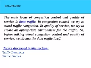
DATA TRAFFIC The main focus of congestion control and quality of service is data traffic. In congestion control we try to avoid traffic congestion. In quality of service, we try to create an appropriate environment for the traffic. So, before talking about congestion control and quality of service, we discuss the data traffic itself. Topics discussed in this section: Traffic DescriptorTraffic Profiles
Traffic descriptors Traffic descriptors are qualitative values that represent a data flow. Average Data Rate: The average data rate is the number of bits sent during a period of time, divided by the number of seconds in that period. We use the following equation:
Peak Data Rate: The peak data rate defines the maximum data rate of the traffic. Maximum Burst Size: Although the peak data rate is a critical value for the network, it can usually be ignored if the duration of the peak value is very short. For example, if data are flowing steadily at the rate of 1 Mbps with a sudden peak data rate of 2 Mbps for just 1 ms, the network probably can handle the situation. However, if the peak data rate lasts 60 ms, there may be a problem for the network. The maximum burst size normally refers to the maximum length of time the traffic is generated at the peak rate. Effective Bandwidth: The effective bandwidth is the bandwidth that the network needs to allocate for the flow of traffic. The effective bandwidth is a function of three values: average data rate, peak data rate, and maximum burst size. The calculation of this value is very complex.
CONGESTION Congestion in a network may occur if the load on the network—the number of packets sent to the network—is greater than the capacity of the network—the number of packets a network can handle. Congestion control refers to the mechanisms and techniques to control the congestion and keep the load below the capacity.
Queues in a router Congestion in a network or internetwork occurs because routers and switches have queues-buffers that hold the packets before and after processing. A router, for example, has an input queue and an output queue for each interface. When a packet arrives at the incoming interface, it undergoes three steps before departing: 1. The packet is put at the end of the input queue while waiting to be checked. 2. The processing module of the router removes the packet from the input queue once it reaches the front of the queue and uses its routing table and the destination address to find the route. 3. The packet is put in the appropriate output queue and waits its turn to be sent.
We need to be aware of two issues. First, if the rate of packet arrival is higher than the packet processing rate, the input queues become longer and longer. Second, if the packet departure rate is less than the packet processing rate, the output queues become longer and longer.
Network performance: Packet delay and throughput as functions of load
CONGESTION CONTROL Congestion control refers to techniques and mechanisms that can either prevent congestion, before it happens, or remove congestion, after it has happened. In general, we can divide congestion control mechanisms into two broad categories: open-loop congestion control (prevention) and closed-loop congestion control (removal).
Open-loop congestion control - Retransmission policy • The retransmission policy and the retransmission timers must be designed to optimize efficiency and at the same time prevent congestion. - Window policy The type of window at the sender may also affect congestion. The selective repeat window is better than go back n window for congestion. • Acknowledgment policy • If the receiver does not acknowledge every packet it receives, it may slow down the sender and help prevent congestion • Discard policy • In audio transmission, if the policy is to discard less sensitive packets when congestion is likely, the quality of sound is still preserved and congestion is prevented. Admission policy Switches first check the resource requirement of a flow before admitting it to the network. A router can deny establishing a virtual circuit connection if there is congestion in the network or if there is a possibility of future congestion.
Closed-loop congestion control - Back pressure • informing the previous upstream router to reduce the rate of outgoing packets • Choke point • is a packet sent by a router to the source to inform it of congestion • is similar to ICMP’s source quench packet
In implicit signaling: There is no communication between the congested node or nodes and the source. The source guesses that there is a congestion somewhere in the network from other symptoms. For example, when a source sends several packets and there is no acknowledgment for a while, one assumption is that the network is congested. The delay in receiving an acknowledgment is interpreted as congestion in the network; the source should slow down. Explicit Signaling: The node that experiences congestion can explicitly send a signal to the source or destination. The explicit signaling method, however, is different from the choke packet method. In the choke packet method, a separate packet is used for this purpose; in the explicit signaling method, the signal is included in the packets that carry data.
Congestion Control in TCP • Congestion window • Today, TCP protocols include that the sender’s window size is not only determined by the receiver but also by congestion in the network • Actual window size = minimum (rwnd, cwnd)
Slow start: exponential increase MSS (max. segment size)
Congestion Control in TCP (cont’d) • Slow start: exponential increase MSS (max. segment size)
Congestion Control in TCP (cont’d) • In the slow start algorithm, the size of the congestion window increases exponentially until it reaches a threshold Start cwnd = 1 After 1 RTT cwnd = 1 x 2 = 2 21 After 2 RTT cwnd = 2 x 2 = 4 22 After 3 RTT cwnd = 4 x 2 = 8 23
Congestion Control in TCP (cont’d) • Congestion avoidance: additive increase • When the size of the congestion window reaches the slow start threshold, in the congestion avoidance algorithm, the size of the congestion window increases additively until congestion is detected
Congestion Control in TCP (cont’d) • Congestion detection: Multiplicative Decrease • Most implementations react differently to congestion detection: • If detection is by time-out, a new slow start phase starts • If detection is by three ACKs, a new congestion avoidance phase starts
Congestion Control in TCP (cont’d) • TCP congestion policy summary
24-6 TECHNIQUES TO IMPROVE QoS we tried to define QoS in terms of its characteristics. In this section, we discuss some techniques that can be used to improve the quality of service.
The Leaky Bucket Algorithm (a) A leaky bucket with water. (b) a leaky bucket with packets.
Note A leaky bucket algorithm shapes bursty traffic into fixed-rate traffic by averaging the data rate. It may drop the packets if the bucket is full.
Note The token bucket allows bursty traffic at a regulated maximum rate.
For each tick of the clock, the system sends n tokens to the bucket. The system removes one token for every cell (or byte) of data sent. For example, if n is 100 and the host is idle for 100 ticks, the bucket collects 10,000 tokens. Now the host can consume all these tokens in one tick with 10,000 cells,