JGR_figures_CAR

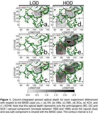
1. Figure 1. Column-integrated aerosol optical depth for each experiment differenced with respect to the BASE case (∆τe ): (a) XA, (b) XBa, (c) XBh, (d) XCa, (e) XCh, and (f ) XChW. Note that this optical depth represents only the anthropogenic (BC, OC and SO4 ) aerosol component (increase between 1950 and 1990) since the natural (dust and sea salt) component is shared with the BASE case. The contour interval is 0.2.

2. Figure 2. All-sky area-average change in JJA anthropogenic aerosol instantaneous direct radiative surface (SFC) and atmospheric (ATM) forcing relative to the BASE case (∆DRF) over India (a-b) and China (c-d) in [W m−2 ]. The total aerosol (natural + anthropogenic) DRF for the BASE case is printed along the bottom of each panel. Here ”net” is defined as shortwave (SW) plus longwave (LW) forcing. Note the differing scales between the LOD (left) and HOD (right) experiments and that the LW forcing is negligible compared to the SW forcing.

3. Figure 3. JJA change in surface temperature (∆Tsfc ) [K] between the BASE case and (a) XA, (b) XBa, (c) XBh, (d) XCa, (e) XCh, and (f ) XChW. (g) Observed mean ∆Tsfc between the 1945-1955 and 1985-1995 decades from the CRU database [Brohan et al., 2006]. Shading and dashed lines indicate ∆Tsfc with a contour interval of 0.5 K, and the thick solid blue and red lines indicate the 90% confidence level.

4. Figure 4. Zonally averaged change in JJA atmospheric temperature (∆Tatm) [K] (shaded) over India (65oE-90oE) between the BASE case and (a) XA, (b) XBa, (c) XBh, (d) XCa, (e) XCh, and (f ) XChW. Change in BC mixing ratio relative to the BASE case (thick black contours) with contour interval of 0.01 µg m−3 in the LOD regime and 0.02 µg m−3 in the HOD regime. Dashed contours indicate the change in short-wave heating rate [K d−1 ] relative to the BASE case with contour intervals of 0.05 and 0.1 for the LOD and HOD regimes, respectively.

5. Figure 5. Zonally averaged JJA change in vertical velocity (∆( −ω) = ∆(−dp/dt)) between the BASE case and experiments over India (65oE-90oE) for (a) XA, (b) XBa, (c) XBh, (d) XCa, (e) XCh, and (f ) XChW. Note that the negative of the vertical pressure velocity is taken such that red shading indicates increased vertical motion and blue shading indicates relative subsidence. The contour interval is 1 hPa s−1 × 10-5.

6. Figure 6. Change in JJA surface pressure (∆PSFC) [hPa] relative to the BASE case for (a) XA, (b) XBa, (c) XBh, (d) XCa, (e) XCh, and (f ) XChW. The thick contours indicate the 90% confidence interval for ∆PSFC. The change in 850 hPa winds relative to the BASE case are plotted as vectors.

7. Figure 7. Change in total JJA precipitation (∆P) relative to the BASE case for (a) XA, (b) XBa, (c) XBh, (d) XCa, (e) XCh, and (f ) XChW. Shading and dashed lines represent ∆P with a contour interval of 1 mm d−1, and thick solid red and blue lines represent the 90% confidence interval.

8. Figure 8. Zonally averaged change in JJA atmospheric temperature (∆Tatm) [K] (shaded) over China (90oE-130oE) between the BASE case and (a) XA, (b) XBa, (c) XBh, (d) XCa, (e) XCh, and (f ) XChW. Change in BC mixing ratio relative to the BASE case (thick black contours) with contour interval of 0.01 µg m−3 in the LOD regime and 0.02 µg m−3 in the HOD regime. Dashed contours indicate the change in short-wave heating rate [K d−1 ] relative to the BASE case with contour intervals of 0.05 and 0.1 for the LOD and HOD regimes, respectively.

9. Figure 9. Zonally averaged JJA change in vertical velocity (∆( −ω) = ∆(−dp/dt)) between the BASE case and experiments over China (90oE-130oE) for (a) XA, (b) XBa, (c) XBh, (d) XCa, (e) XCh, and (f ) XChW. Note that the negative of the vertical pressure velocity is taken such that red shading indicates increased vertical motion and blue shading indicates relative subsidence. The contour interval is 1 hPa s−1 × 10-5.

10. Figure 10. Percent change in total precipitation rate relative to the BASE case ((EXP- BASE)/BASE) × 100 over China for: (a) XA, (b) XBa, (c) XBh, (d) XCa, (e) XCh, and (f ) XChW. (g) Observed percent change in total precipitation between the 1985-1995 decade and the 1945-1955 decade from the CRU database [Brohan et al., 2006]. Shading and dashed contours represent a 5% change in precipitation, and the thick solid red and blue contours represent the 90% confidence interval.

11. Land-area average JJA change in total cloud amount [%] relative to the BASE case for (a) XA, (b) XBa, (c) XBh, (d) XCa, (e) XCh, and (f) XChW. Note that cloud amount refers to the change in the spatially averaged frequency of occurrence of clouds (Wetherald and Manabe , 1988; Erlick et al., 2006). Dashed contours represent a 2% change in total cloud amount, and the thick solid red and blue contours represent the 90% confidence interval.

12. Land-area average JJA change in low cloud amount [%] relative to the BASE case for (a) XA, (b) XBa, (c) XBh, (d) XCa, (e) XCh, and (f) XChW. Low clouds are defined as those forming between 680 and 1000 hPa. Note that cloud amount refers to the change in the spatially averaged frequency of occurrence of clouds (Wetherald and Manabe , 1988; Erlick et al., 2006). Contours represent a 1% change in low cloud amount.

13. Land-area average JJA vertical profile of total, low, mid, and high cloud amount. Low clouds are defined as those forming between 680 and 1000 hPa, middle clouds form between 440 and 680 hPa, and high clouds form between 10 and 440 hPa. Note that cloud amount refers to the change in the spatially averaged frequency of occurrence of clouds (Wetherald and Manabe , 1988; Erlick et al., 2006).

14. Land-area average JJA change in total, low, mid, and high cloud amount relative to the BASE case. Low clouds are defined as those forming between 680 and 1000 hPa, middle clouds form between 440 and 680 hPa, and high clouds form between 10 and 440 hPa. Note that cloud amount refers to the change in the spatially averaged frequency of occurrence of clouds (Wetherald and Manabe , 1988; Erlick et al., 2006).