Scattering Power in Monte Carlo Transport
Learn about scattering power and its role in Monte Carlo Transport methods for dosimetry and nuclear physics simulations. Discover how to calculate scattering power and its impact on proton transport accuracy.


Scattering Power in Monte Carlo Transport
E N D
Presentation Transcript
Scattering Power arXiv:0908.1413v1 [physics.med-ph] 10 Aug 2009andMed. Phys. 37(1) (2010) 352-367 We thank N. Kanematsu, U. Schneider and M. Hollmark for discussions of their work and L. Urban (CERN) for providing test data on the step size dependence of Geant4. We thank Harvard University, the Physics Department, and the Lab for Particle Physics and Cosmology for ongoing support. You can get a copy of the article by Googling arXiv and following links.
Questions What is scattering power (T ) ? Why do we need it ? What happens if we try to derive T directly ? What is the single scattering correction ? What is the correct theory of multiple Coulomb scattering in the Gaussian approximation ? How can we use that to derive the correct form of T ? How can we parameterize that to obtain a simple formula for T ? In practical problems, does the formula for T make any difference ?
Monte Carlo Transport 1 2 3 4 x 0 In dosimetry all practical Monte Carlos are condensed history MC’s. The target geometry is divided into small steps. Given incoming positions, slopes, energy, we estimate an interaction point. At that point we compute the ms deflection We use that as the rms of a distribution from which we pick a random deflection. We project to the next boundary and compute outgoing positions, slopes, and energy. We repeat for all steps and 106 protons (‘histories’). We accumulate the distribution of y at x and find its rms width.
Δθ Δx Integrating MCS in a Monte-Carlo Method 1: treat Δx as an MCS problem de novo (respecting pv, of course). Compute the parameters of a probability distribution function (PDF) and pick Δθ at random using that PDF. This method usually does not converge (Geant4 ?) (Note: Molière should converge but only if we do it exactly which is very slow.) Method 2: use a ‘scattering power’ function T ≡ d<θ2>/dx . Compute σ = <θ2>1/2 = (T Δx)1/2 and pick Δθ at random from a Gaussian PDF having that σ. This method converges by construction, but may be quite wrong depending on your choice of T(x) (MCNPX ?). The Gaussian approximation is built in.
Convergence Studies σ of the outgoing angular distribution when 158.6 MeV protons enter 20.196 g/cm2 (1.78 cm) of Pb, as a function of the number of steps in a Monte Carlo calculation. ‘BG’ curves from BG toy Monte Carlo. Geant4 curve by courtesy of L. Urban. Experimental point from Gottschalk et al., NIM B74 (1993) 467-490 .
Deterministic (Fermi-Eyges) Transport 1 2 3 4 x 0 yrms midpoint rule
What is scattering power, really ? Unlike stopping theory, which begins with stopping power - dE/dx, multiple scattering theory does not flow naturally from a differential description. The reason is profound: we can speak of energy loss even in an atomic monolayer, but not of multiple scattering. But we need a differential description to do proton transport. Therefore we seek a posteriori a differential description of Molière/Fano/Hanson theory: a function T which, when integrated, will reproduce the correct theory for a single slab to a sufficiently good approximation. T is necessarily approximate. Some formulas are more accurate and/or more useful than others. Having found a T that works well for single slabs we may hope that it works for mixed slabs, but we cannot know for sure. There is no accurate theory, and there are no experimental data. Monte Carlo is not a test!
The Single Scattering Correction H. Bichsel, Phys. Rev. 112 (1958) 182-185 He bombarded targets of Al, Ni, Ag and Au with protons ranging from 0.77 to 4.8 MeV, Van de Graaff accelerator. Graph shows the Gaussian coreand the start of the single scattering tail. The competition between them, as you increase target thickness, affects the rate of increase of the Gaussian width. This effect, a natural part of the full theory, becomes the ‘single scattering correction’ when we try to write down a scattering power. place
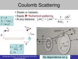
Rossi’s Derivation Rossi first gives a simplified Rutherford derivation of the single scattering probability, per unit target thickness and per unit solid angle, from an unscreened point charge, namely 1/χ4 breaks down for distant collisions (very small scattering angle) because the nucleus is screened by electrons. That happens near ? It also breaks down for very close collisions (large scattering angle) because the nucleus is not a point charge. That happens near ? χ2 χ1
Rossi’s Derivation (cont.) Rossi now assumes that the mean squared angle at (x + dx) equals its value at x plus the mean squared angle of scattering in dx. This step is equivalent to assuming the MCS process is exactly Gaussian. It leads to He then defines Later, Brahme called this quantity the mass scattering power T/ρ and made the analogy with mass stopping power S/ρ . Note that in Rossi, x is expressed in g/cm2 : his x is our ρx . Absorbing ρ in x or other quantities such as X0 becomes very inconvenient when dealing with mixed slabs. Instead of doing that we simply regard ρ and other material properties as piecewise constant functions of depth x (cm).
χ2 χ1 Rossi’s Derivation (cont.) To do the integral in closed form one must assume some simple behavior for Ξ below χ1 and above χ2. Rossi does this two different ways. The less accurate, which unfortunately became known as the ‘Rossi formula’, assumes that Ξ is 0 below χ1 and above χ2. Then the integral is easy, and with the aid of one eventually finds (in our notation): X0 is the radiation length of the material. To find the net MCS angle in a finite slab, we must integrate TFR over x, taking into account the decrease of pv (momentum × speed) as the protons slow down:
The Fermi-Rossi Scattering Power TFR TFR is simple but it does not work very well. Here we compare its integral with the right answer. θ0 is far too large for thin targets, and it has the wrong material dependence.
χ2 χ1 Rossi’s Derivation (cont.) Rossi later makes the more reasonable assumption that Ξ(χ) ≈ 1/(χ2+χ12)2 below χ1 . The integral is a bit harder but still analytic : This is the scattering power given in ICRU Report 35 (1984) except that the form given there only applies to electrons. For protons it can be simplified by introducing a ‘scattering length’ XS defined by whereupon identical in form and kinematic dependence to TFR. The result is greatly improved material dependence but the same problem for thin targets.
The ‘ICRU Report 35’ Scattering Power TIC For protons, TIC is as simple as TFR and considerably improved. We will use it as a building block, adding a single scattering correction (nonlocal term) to improve accuracy for thin scatterers.
The Real Answer Gottschalk et al. NIM B74 (1993) 467-490. Molière/Fano/Hanson theory predicts θ0 to a few percent over a wide range of target materials and normalized target thicknesses. We can use it to deduce the correct numerical value of T for any useful materials and thicknesses.
Finding the Real T Suppose we want to find T in Be at 20 Mev. That question is not well posed, because a point where the proton has 20 MeV can have any amount of overlying material x (cm). Two cases are shown at right. For any given case we can find the correct value of T by differentiating Molière/Fano/Hanson theory numerically (below). However, that involves a lengthy calculation and therefore does not directly yield a useful expression for T. We need to parameterize it somehow. Be x1 0 Be x2 0 20 MeV
The Single Scattering Correction The result for 20 MeV protons in three materials, over a range of x’s (total thickness) relevant to proton therapy calculations. To improve the graph we have plotted mass scattering power vs. normalized thickness. TFR and TIC are local; they do not care about overlying material. THanson is nonlocal . The single scattering correction is larger, the thinner the degrader. We will now express THanson as TIC times an approximate single scattering correction and call the result TdM .
The Øverås-Schneider Scattering Power Schneider et al., Z. Med. Phys. 11 (2001) 110-118 propose a scattering power which is TFR multiplied by a single scattering correction in the form of a polynomial in t ≡ x/R1. For mixed slabs, regard t as that normalized depth which would result if the proton were degraded in the current material.
Kanematsu’s Scattering Power TdH N. Kanematsu, NIM B266 (2008) 5056-5062 describes a differential form of Highland’s formula, obtained by multiplying TFR by a single scattering correction factor which is logarithmic in a new pathlength integral l , the total x/X0 traversed by the proton. This generalizes easily to mixed slabs.
The Øverås Approximation E ≡ kinetic energy H. Øverås, CERN Yellow Report 60-18 (1960). If we express the single scattering correction directly as a function of x/R1 it will not generalize gracefully to mixed slabs (different materials). The Øverås approximation lets us get around that.
The Single Scattering Correction Parameterized Do the whole calculation for Be, Cu, and Pb, four local energies, and the whole interesting range of log10(1-(pv/p1v1)2). Plot THanson/TIC and fit with a line whose coefficients are themselves linear in log10(pv/MeV).
Experimental Test, Polystyrene data/θHanson (Gottschalk et al. NIM B74 (1993) 467-490) along with results from all known formulas for Tincluding another by Kanematsu (‘corrected Rossi’) and the generalized Highland formula Formulas for all are in the paper.
Experimental Test, Lead (Pb) The same for Pb.
Does any of this matter ? Not in water. Except for TFR and THO (which is simply wrong) beam spreading in light materials is remarkably insensitive to the formula for T . That is fortunate because it means that dose reconstruction algorithms tend to be insensitive to T. Thus, the ‘back end’ of a Monte Carlo simulation is insensitive to the MCS model.
Beam Spreading in H2O and Pb Evolution of Fermi-Eyges beam ellipses in near stopping targets of water (left) and Pb (right) for 127 MeV protons. Shows that the insensitivity of beam spreading to T is a fortuitous property of water-like materials. If we were computing slit scattering in brass or Cerrobend, T would make some difference.
M1 M2 M3 Pb Lexan air E1 R1 p1v1 E R pv Δx x1 x2 x3 x 0 But suppose we have an upstream modulator ... ... as in the standard IBA proton nozzle.
Beam rms width at the exit of the Pb/Lexan/air stack (that is, at the second scatterer) for each step of the ‘modulator’ and for six scattering powers. If the actual width does not match the design width (3.5 cm) the dose at the patient will not be flat. Open squares are MC results, which agree with Fermi-Eyges. The front end (beam line) of a proton MC calculation is sensitive to the MCS model !
Answers Scattering power (T ) is a differential approximation to MCS theory. We need it for charged particle transport, deterministic or Monte Carlo. If we try to start with a differential form we get the wrong answer, especially for thin scatterers, because that assumes the Gaussian approximation is exact. To improve simple (local) formulas for T we need a ‘single scattering correction’. The correct theory of multiple Coulomb scattering in the Gaussian approximation is Molière/Fano/Hanson theory. The correct numerical value of T can be obtained for any single slab problem by differentiating MFH theory numerically, but that is not useful by itself . With the aid of the Øverås approximation T can be written in a simple form applicable to mixed slabs. The single scattering correction is expressed as a logarithmic function of current pv and initial pv . (An accurate T is necessarily non-local.) In many problems, T (that is, the MCS model) makes no difference, but sometimes it does!