Download
1 / 20
220 likes | 370 Views
Utilization of Observations at the Russian Drifting Stations “North Pole” for Improved Description of Air–Sea-Ice-Ocean Interactions in the Arctic Ocean A. Makshtas, Sokolov V. , S. Shutilin, V. Kustov, N. Zinoviev, Arctic and Antarctic Research Institute, Saint Petersburg, Russia,

E N D
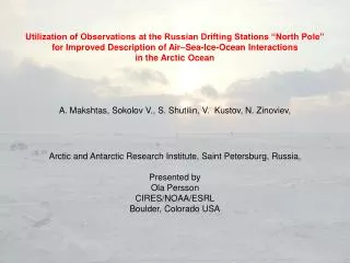
Utilization of Observations at the Russian Drifting Stations “North Pole” for Improved Description of Air–Sea-Ice-Ocean Interactions in the Arctic Ocean A. Makshtas, Sokolov V., S. Shutilin, V. Kustov, N. Zinoviev, Arctic and Antarctic Research Institute, Saint Petersburg, Russia, Presented by Ola Persson CIRES/NOAA/ESRL Boulder, Colorado USA
Russian drifting stations “North Pole” in 2003-2012 Barrow Greenland Canada Basin Chukchi Sea Wrangell Is. Pevek Spitsbergen Barents Sea Tiksi
Science Issues Being Studied with “North Pole” station data • Atmospheric • Cryospheric • Oceanic • Greenhouse Gas
Radiosound Overview of observations, organized at drifting station “North Pole – 39” and future “North Pole” stations aerostat Unmanned plane MAWS-420 GPS and GLONAS systems for ice drift calculations Inlets of ozone, carbon dioxide, methane and radioactivity analyzers Polygon 80x100 m for mass balance and dynamic studies Lidar Ice thickness measurements Radiation Carbon dioxide flux measurements Precipitation gauge Weather shed Total ozone Echo-sounder Snow height Spectrometer “Ramses” IMB buoy Transmitter IMB Thermo chain IMB Echo-sounder emitter Long ranger ADCP WH LP 757 ADCP WHS 300 Ice thickness submersible vehicle 2 SBE 37SM MicroCat 3 SBE 19 profilers Current meter RCM Grid Juday
Atmospheric Science Issues • 1) characterizing low-level inversions • 2) cloud characteristics (cloud fraction, height; measurement technique variability) • 3) atmospheric boundary layer thermal structure – variability processes • 4) atmospheric O3 • - surface-layer/boundary layer • - stratosphere – Arctic “ozone holes” • 5) measurement techniques (e.g., clouds, skin temperature) • 6) validation of models: mesoscale (WRF), RCMs and reanalyses - T, Td, cloud fraction, BL thermal & kinematic structure - surface characteristics • 7) parameterization validations - downwelling SW and LW radiation, incl. impact of clouds - turbulent fluxes in stable boundary layer - atmospheric boundary layer, for forcing sea-ice models
Clear skies Monthly mean profiles (April 2008; NP-36) of air temperature from radiosoundings and calculated by HIRHAM4 (AWI Regional Climate Model) and ECMWF (ERA-Interim Reanalysis?) ECMWF radiosondes Height (m) HIRHAM Cloudy Skies T (deg C) Clear Skies Observations: surface-based inversion Models: shallow mixed layers, too warm Ts radiosondes HIRHAM Height (m) ECMWF Cloudy Skies Observations: surface mixed layer Models: surface mixed layers, too warm ML, inversions too weak & too deep T (deg C)
Detailed atmospheric boundary-layer processes: New approach with microwave 56.7 GHz temperature profiler at “North Pole 39” (April 2012) Descent of inversion top Height (m) Hour mixed layer to 300 m surface-based inversion
Ozone studies at “North Pole” drifting stations (March 2011, NP-38) Ozone concentration in atmospheric surface layer in spring Evidence of “Ozone hole” in the Central Arctic (March 2011) Total cloudiness (in tenths), from ceilometer data and visual observations (Nov. 2008, NP-36) visual NOAAceilometer
Comparison air surface temperature (T) and total cloudiness (N)between NP and NCEP/NCAR Reanalysis data for 2007-2008
Cryospheric Science Issues • spatial and temporal variability of spectral albedo of snow/ice – transects of snow depth, density, morphology, spectral albedo (e.g., every 2nd day) • spatial and temporal variability of sea-ice surface characteristics (e.g., leads, meltponds, etc) • spatial and temporal variability of ice thickness • sub-surface ice structure • validation of modeled snow depth and ice thickness distributions
Transect average spectral albedo for day 98 to 215 (NP-36) and day 115 – 191 (NP 35)
Ice floe characteristics near drifting station “North Pole 38” in winter UAS – the new instrument for study of sea ice cover Weight – 3.5 kg, wingspan – 1.4 m, range of flight speed 60 - 100 km/h, altitudes - 50 - 3000 m. October April December
Ice floe characterization of summer melt - “North Pole 38” June 19 June 29 July 16 August 30
Manual ice thickness measurements (NP-36) min ~ 195 cm min ~ 78 cm Distance (m) max ~ 131 cm max ~ 236 cm Distance (m) Distance (m) 80 x 100 m grid of 35 points September 30, 2008 May 27, 2009 - mean growth of 1.3 m - thickness range decreased during winter from 63 cm to 41 cm (thinner ice regions grew faster) Ice thickness (m) Date Mean thickness Minimum thickness Maximum thickness
Comparison of measured and modeled snow and ice thickness evolutions - AARI dynamic-thermodynamic sea-ice model (Makshtas et al., 2003; JGR) with observational external forcing Snow Ice NP-35 model model Snow depth (m) measurements Ice thickness (m) measurements Year Day Year Day NP-36 model model Ice thickness (m) measurements Snow depth (m) measurements Year Day Year Day
Oceanic Science Issues • Temporal variability of solar radiation penetration of sea ice • Spectral and depth redistribution of solar radiation
Solar energy penetration of sea-ice and redistribution in upper ocean as function of wavelength and month .02-.09 W m-2 April mW/(m2 nm) May Depth (m) June 2.2 - 7.2 W m-2 mW/(m2 nm) July Depth (m) Wavelength (nm)
Greenhouse Gas Science Issues • 1) Understanding greenhouse gas concentrations and fluxes – CO2
Comparison of seasonal variability of CO2 concentration at drifting stations NP-35, NP-36 and Observatories in Barrow and Alert Monthly mean CO2 concentration Direct measurements of CO2 flux with automatic chamber Monthly relative CO2 variability (s/m) a) during summer and early autumn, ice-free Arctic shelf seas serve as a sink for atmospheric CO2. b) in late autumn and winter, cooling seawater is CO2source to atmosphere. Question: what is the net role of sea ice in modulating or otherwise affecting this CO2 exchange? (Makshtas et al 2011; AMS Conf. on Polar Meteor. & Ocean.)
Scope of Future Work at Russian North Pole Stations • Study of polar cloudiness • 2. Detailed investigations of atmospheric surface and boundary layers- studies of stable boundary layers- improve/validate parameterizations of BL for forcing sea-ice models- improve/validate mesoscale models, esp. surface characteristics • 3. Investigate spatial characteristics and radiative properties of sea ice cover • 4. Comprehensive study of atmospheric ozone (from surface to stratosphere) • 5. Study of greenhouse gas concentrations and ice/ocean fluxes