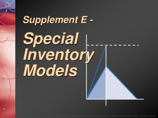
Supplement E - Special Inventory Models
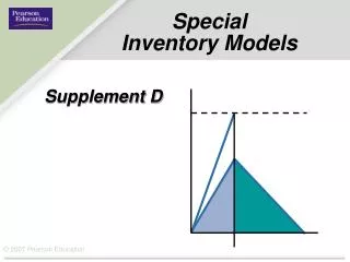
Supplement E - Special Inventory Models. Production quantity. Q. Demand during production interval. I max. On-hand inventory. Maximum inventory. p – d. Time. Production and demand. Demand only. TBO. Figure E.1. Special Inventory Models. I max = ( p – d ) = Q ( ).

Supplement E - Special Inventory Models
E N D
Presentation Transcript
Production quantity Q Demand during production interval Imax On-hand inventory Maximum inventory p – d Time Production and demand Demand only TBO Figure E.1 Special Inventory Models
Imax = (p – d) = Q( ) p – d p Q p Special Inventory Models Production quantity Q Demand during production interval Imax On-hand inventory Maximum inventory p – d Time Production and demand Demand only TBO
Imax 2 D Q C = (H) + (S) Special Inventory Models Production quantity Q Demand during production interval Imax On-hand inventory Maximum inventory p – d Time Production and demand Demand only TBO
Production quantity Q Demand during production interval Imax On-hand inventory Maximum inventory C = ( ) + (S) Q p – d 2 p D Q p – d Time Production and demand Demand only TBO Special Inventory Models
Production quantity Q Demand during production interval Imax On-hand inventory Maximum inventory p p – d 2DS H ELS = p – d Time Production and demand Demand only TBO Figure E.1 Special Inventory Models
Special Inventory Models Economic Production Lot Size Demand = 30 barrels/day Setup cost = $200 Production rate = 190 barrels/day Annual holding cost = $0.21/barrel Annual demand = 10,500 barrels Plant operates 350 days/year 2(10,500)($200) $0.21 190 190 – 30 ELS = ELS = 4873.4 barrels Example E.1
Special Inventory Models Economic Production Lot Size Demand = 30 barrels/day Setup cost = $200 Production rate = 190 barrels/day Annual holding cost = $0.21/barrel Annual demand = 10,500 barrels Plant operates 350 days/year ELS = 4873.4 barrels C = ( )(H) + (S) Q p – d 2 p D Q Example E.1
Special Inventory Models Economic Production Lot Size Demand = 30 barrels/day Setup cost = $200 Production rate = 190 barrels/day Annual holding cost = $0.21/barrel Annual demand = 10,500 barrels Plant operates 350 days/year ELS = 4873.4 barrels C = ( ) ($0.21) + ($200) 10,500 4873.4 4873.4 190 – 30 2 190
Special Inventory Models Economic Production Lot Size Demand = 30 barrels/day Setup cost = $200 Production rate = 190 barrels/day Annual holding cost = $0.21/barrel Annual demand = 10,500 barrels Plant operates 350 days/year ELS = 4873.4 barrels C = $430.91 + $430.91 Example E.1
Special Inventory Models Economic Production Lot Size Demand = 30 barrels/day Setup cost = $200 Production rate = 190 barrels/day Annual holding cost = $0.21/barrel Annual demand = 10,500 barrels Plant operates 350 days/year ELS = 4873.4 barrels C = $861.82 ELS D TBOELS = (350 days/year) Example E.1
Economic Production Lot Size Special Inventory Models Demand = 30 barrels/day Setup cost = $200 Production rate = 190 barrels/day Annual holding cost = $0.21/barrel Annual demand = 10,500 barrels Plant operates 350 days/year ELS = 4873.4 barrels C = $861.82 TBOELS = 162.4, or 162 days Example E.1
Special Inventory Models Economic Production Lot Size Demand = 30 barrels/day Setup cost = $200 Production rate = 190 barrels/day Annual holding cost = $0.21/barrel Annual demand = 10,500 barrels Plant operates 350 days/year ELS = 4873.4 barrels ELS p Production time = C = $861.82 TBOELS = 162.4, or 162 days Example E.1
Special Inventory Models Economic Production Lot Size Demand = 30 barrels/day Setup cost = $200 Production rate = 190 barrels/day Annual holding cost = $0.21/barrel Annual demand = 10,500 barrels Plant operates 350 days/year ELS = 4873.4 barrels Production time = 25.6, or 26 days C = $861.82 TBOELS = 162.4, or 162 days Example E.1
Special Inventory Models Economic Production Lot Size Figure E.2
0 100 200 300 0 100 200 300 Purchase quantity (Q) Purchase quantity (Q) Special Inventory Models Quantity Discounts Figure E.3 EOQ 4.00 EOQ 3.50 EOQ 3.00 C for P = $4.00 C for P = $3.50 C for P = $3.00 Total cost (dollars) PD for P = $4.00 Total cost (dollars) PD for P = $3.50 PD for P = $3.00 First price break Second price break First price break Second price break (a) Total cost curves with purchased materials added (b) EOQs and price break quantities
Order Quantity Price per Unit 0 – 299 $60.00 300 – 499 $58.80 500 or more $57.00 2DS H Special Inventory Models Quantity Discounts Annual demand = 936 units Ordering cost = $45 Holding cost = 25% of unit price EOQ57.00 = 2(936)(45) 0.25(57.00) EOQ57.00 = Example E.2
Order Quantity Price per Unit 0 – 299 $60.00 300 – 499 $58.80 500 or more $57.00 Special Inventory Models Quantity Discounts Annual demand = 936 units Ordering cost = $45 Holding cost = 25% of unit price EOQ57.00 = 77 units EOQ58.80 = 76 units Example E.2
Order Quantity Price per Unit 0 – 299 $60.00 300 – 499 $58.80 500 or more $57.00 Special Inventory Models Quantity Discounts Annual demand = 936 units Ordering cost = $45 Holding cost = 25% of unit price EOQ57.00 = 77 units EOQ58.80 = 76 units EOQ60.00 = 75 units Example E.2
Order Quantity Price per Unit 0 – 299 $60.00 300 – 499 $58.80 500 or more $57.00 D Q Q 2 C = (H) + (S) + PD Special Inventory Models Quantity Discounts Annual demand = 936 units Ordering cost = $45 Holding cost = 25% of unit price EOQ57.00 = 77 units EOQ58.80 = 76 units EOQ60.00 = 75 units Example E.2
Order Quantity Price per Unit 0 – 299 $60.00 300 – 499 $58.80 500 or more $57.00 Special Inventory Models Quantity Discounts Annual demand = 936 units Ordering cost = $45 Holding cost = 25% of unit price EOQ57.00 = 77 units EOQ58.80 = 76 units EOQ60.00 = 75 units 936 75 75 2 C75 = [(0.25)($60.00)] + ($45) + $60.00(936) C75 = $57,284 Example E.2
Order Quantity Price per Unit 0 – 299 $60.00 300 – 499 $58.80 500 or more $57.00 Special Inventory Models Quantity Discounts Annual demand = 936 units Ordering cost = $45 Holding cost = 25% of unit price EOQ57.00 = 77 units EOQ58.80 = 76 units EOQ60.00 = 75 units C75 = $57,284 936 300 300 2 C300 = [(0.25)($58.80)] + ($45) + $58.80(936)
Order Quantity Price per Unit 0 – 299 $60.00 300 – 499 $58.80 500 or more $57.00 Special Inventory Models Quantity Discounts Annual demand = 936 units Ordering cost = $45 Holding cost = 25% of unit price EOQ57.00 = 77 units EOQ58.80 = 76 units EOQ60.00 = 75 units C75 = $57,284 C300 = $57,382 Example E.2
Order Quantity Price per Unit 0 – 299 $60.00 300 – 499 $58.80 500 or more $57.00 Special Inventory Models Quantity Discounts Annual demand = 936 units Ordering cost = $45 Holding cost = 25% of unit price EOQ57.00 = 77 units EOQ58.80 = 76 units EOQ60.00 = 75 units C75 = $57,284 C300 = $57,382 936 500 500 2 C500 = [(0.25)($57.00)] + ($45) + $57.00(936) Example E.2
Order Quantity Price per Unit 0 – 299 $60.00 300 – 499 $58.80 500 or more $57.00 Quantity Discounts Special Inventory Models Annual demand = 936 units Ordering cost = $45 Holding cost = 25% of unit price EOQ57.00 = 77 units EOQ58.80 = 76 units EOQ60.00 = 75 units C75 = $57,284 C300 = $57,382 C500 = $56,999 Example E.2
Order Quantity Price per Unit 0 – 299 $60.00 300 – 499 $58.80 500 or more $57.00 Special Inventory Models Quantity Discounts Annual demand = 936 units Ordering cost = $45 Holding cost = 25% of unit price EOQ57.00 = 77 units EOQ58.80 = 76 units EOQ60.00 = 75 units C75 = $57,284 C300 = $57,382 C500 = $56,999 Example E.2
Special Inventory Models Figure E.4
Demand 10 20 30 40 50 Demand Probability 0.2 0.3 0.3 0.1 0.1 D Q 10 20 30 40 50 10 $100 $100 $100 $100 $100 20 30 40 50 Special Inventory Models One-Period Decisions Profit per ornament during season = $10 Loss per ornament after season = $5 For Q≤D Payoff = pQ Example E.3
Demand 10 20 30 40 50 Demand Probability 0.2 0.3 0.3 0.1 0.1 D Q 10 20 30 40 50 10 $100 $100 $100 $100 $100 20 200 200 200 200 30 300 300 300 40 400 400 50 500 Special Inventory Models One-Period Decisions Profit per ornament during season = $10 Loss per ornament after season = $5 For Q≤D Payoff = pQ Example E.3
Demand 10 20 30 40 50 Demand Probability 0.2 0.3 0.3 0.1 0.1 D Q 10 20 30 40 50 10 $100 $100 $100 $100 $100 20 200 200 200 200 30 300 300 300 40 400 400 50 500 Special Inventory Models One-Period Decisions Profit per ornament during season = $10 Loss per ornament after season = $5 For Q > D Payoff = pD – I(Q – D) Example E.3
Demand 10 20 30 40 50 Demand Probability 0.2 0.3 0.3 0.1 0.1 D Q 10 20 30 40 50 10 $100 $100 $100 $100 $100 20 200 200 200 200 30 300 300 300 40 400 400 50 500 Special Inventory Models One-Period Decisions Profit per ornament during season = $10 Loss per ornament after season = $5 For Q > D Payoff = ($10)(30) – ($5)(40 – 30) Example E.3
Demand 10 20 30 40 50 Demand Probability 0.2 0.3 0.3 0.1 0.1 D Q 10 20 30 40 50 10 $100 $100 $100 $100 $100 20 200 200 200 200 30 300 300 300 40 250 400 400 50 500 Special Inventory Models One-Period Decisions Profit per ornament during season = $10 Loss per ornament after season = $5 For Q > D Payoff = $250 Example E.3
Demand 10 20 30 40 50 Demand Probability 0.2 0.3 0.3 0.1 0.1 D Q 10 20 30 40 50 10 $100 $100 $100 $100 $100 20 50 200 200 200 200 30 0 150 300 300 300 40 –50 100 250 400 400 50 –100 50 200 350 500 Special Inventory Models One-Period Decisions Profit per ornament during season = $10 Loss per ornament after season = $5 For Q > D Payoff = pD – I(Q – D) Example E.3
Special Inventory Models Figure E.5
Demand 10 20 30 40 50 Demand Probability 0.2 0.3 0.3 0.1 0.1 Expected payoff30 = D Q 10 20 30 40 50 10 $100 $100 $100 $100 $100 20 50 200 200 200 200 30 0 150 300 300 300 40 –50 100 250 400 400 50 –100 50 200 350 500 Special Inventory Models One-Period Decisions Profit per ornament during season = $10 Loss per ornament after season = $5 Example E.3
Demand 10 20 30 40 50 Demand Probability 0.2 0.3 0.3 0.1 0.1 Expected payoff30 = 0.2($0) + 0.3($150) + 0.3($300) + 0.1($300) + 0.1($300) D Q 10 20 30 40 50 10 $100 $100 $100 $100 $100 20 50 200 200 200 200 30 0 150 300 300 300 40 –50 100 250 400 400 50 –100 50 200 350 500 One-Period Decisions Special Inventory Models Profit per ornament during season = $10 Loss per ornament after season = $5 Example E.3
Demand 10 20 30 40 50 Demand Probability 0.2 0.3 0.3 0.1 0.1 Expected payoff30 = $195 Special Inventory Models One-Period Decisions Profit per ornament during season = $10 Loss per ornament after season = $5 D Q 10 20 30 40 50 Expected Payoff 10 $100 $100 $100 $100 $100 20 50 200 200 200 200 30 0 150 300 300 300 195 40 –50 100 250 400 400 50 –100 50 200 350 500 Example E.3
Demand 10 20 30 40 50 Demand Probability 0.2 0.3 0.3 0.1 0.1 Special Inventory Models One-Period Decisions Profit per ornament during season = $10 Loss per ornament after season = $5 D Q 10 20 30 40 50 Expected Payoff 10 $100 $100 $100 $100 $100 $100 20 50 200 200 200 200 170 30 0 150 300 300 300 195 40 –50 100 250 400 400 175 50 –100 50 200 350 500 140 Figure E.6
Demand 10 20 30 40 50 Demand Probability 0.2 0.3 0.3 0.1 0.1 Special Inventory Models One-Period Decisions Profit per ornament during season = $10 Loss per ornament after season = $5 D Q 10 20 30 40 50 Expected Payoff 10 $100 $100 $100 $100 $100 $100 20 50 200 200 200 200 170 30 0 150 300 300 300 195 40 –50 100 250 400 400 175 50 –100 50 200 350 500 140 Figure E.6