Inventory Models
Inventory Models. Overview of Inventory Issues. Proper control of inventory is crucial to the success of an enterprise. Typical inventory problems include: Basic inventory – Planned shortage Quantity discount – Periodic review Production lot size – Single period

Inventory Models
E N D
Presentation Transcript
Overview of Inventory Issues • Proper control of inventory is crucial to the success of an enterprise. • Typical inventory problems include: • Basic inventory – Planned shortage • Quantity discount – Periodic review • Production lot size – Single period • Inventory models are often used to develop an optimal inventory policy, consisting of: • An order quantity, denoted Q. • A reorder point, denoted R.
Type of Costs in Inventory Models • Inventory analyses can be thought of as cost-control techniques. • Categories of costs in inventory models: • Holding (carrying costs) • Order/ Setup costs • Customer satisfaction costs • Procurement/Manufacturing costs
Ch = Annual holding cost per unit in inventory H = Annual holding cost rate C = Unit cost of an item Ch = H * C Type of Costs in Inventory Models • Holding Costs (Carrying costs): These costs depend on the order size • Cost of capital • Storage space rental cost • Costs of utilities • Labor • Insurance • Security • Theft and breakage • Deterioration or Obsolescence
Type of Costs in Inventory Models • Order/Setup Costs These costs are independent of the order size. • Order costs are incurred when purchasing a good from a supplier. They include costs such as • Telephone • Order checking • Labor • Transportation • Setup costs are incurred when producing goods for sale to others. They can include costs of • Cleaning machines • Calibrating equipment • Training staff Co = Order cost or setup cost
Type of Costs in Inventory Models • Customer Satisfaction Costs • Measure the degree to which a customer is satisfied. • Unsatisfied customers may: • Switch to the competition (lost sales). • Wait until an order is supplied. • When customers are willing to wait there are two types of costs incurred: Cb= Fixed administrative costs of an out of stock item ($/stockout unit). Cs = Annualized cost of a customer awaiting an out of stock item($/stockout unit per year).
Type of Costs in Inventory Models • Procurement/Manufacturing Cost • Represents the unit purchase cost (including transportation) in case of a purchase. • Unit production cost in case of in-house manufacturing. C = Unit purchase or manufacturing cost.
Demand in Inventory Models • Demand is a key component affecting an inventory policy. • Projected demand patterns determine how an inventory problem is modeled. • Typical demand patterns are: • Constant over time (deterministic inventory models) • Changing but known over time (dynamic models) • Variable (randomly) over time (probabilistic models) D = Demand rate (usually per year)
Inventory Classifications Inventory can be classified in various ways: Items are classified by their relative importance in terms of the firm’s capital needs. Used typically by accountants at manufacturing firms. Enables management to track the production process. Management of items with short shelf life and long shelf life is very different
Review Systems • Two types of review systems are used: • Continuous review systems. • The system is continuously monitored. • A new order is placed when the inventory reaches a critical point. • Periodic review systems. • The inventory position is investigated on a regular basis. • An order is placed only at these times.
Review Systems continuous review system • Continuous review systems. • The system is continuously monitored. • A new order is placed when the inventory reaches a critical point. • EOQ
ALLEN APPLIANCE COMPANY (AAC) • AAC wholesales small appliances. • AAC currently orders 600 units of the Citron brand juicer each time inventory drops to 205 units. • Management wishes to determine an optimal ordering policy for the Citron brand juicer
ALLEN APPLIANCE COMPANY (AAC) • Data • Co = $12 ($8 for placing an order) + (20 min. to check)($12 per hr) • Ch = $1.40 [HC = (14%)($10)] • C = $10. • H = 14% (10% ann. interest rate) + (4% miscellaneous) • D = demand information of the last 10 weeks was collected:
ALLEN APPLIANCE COMPANY (AAC) • Data • The constant demand rate seems to be a good assumption. • Annual demand = (120/week)(52weeks) = 6240 juicers.
AAC – Solution:EOQ and Total Variable Cost • Current ordering policy calls for Q = 600 juicers. TV( 600) = (600 / 2)($1.40) + (6240 / 600)($12) = $544.80 EOQ = sqrt((2*6240*12)/1,4) = 327,065 = 327 Savings of 16% Savings of 16% TV(327) = (327 / 2)($1.40) + (6240 / 327) ( $12) = $457.89
AAC – Solution:Reorder Point and Total Cost • Under the current ordering policy AAC holds 13 units safety stock (how come? observe): • AAC is open 5 day a week. • The average daily demand = 120/week/5 = 24 juicers. • Lead time is 8 days. Lead time demand is (8)(24) = 192 juicers. • Reorder point without Safety stock = LD = 192. • Current policy: R = 205. • Safety stock = 205 – 192 = 13. • For safety stock of 13 juicers the total cost is TC(327) = 457.89 + 6240($10) + (13)($1.40) = $62,876.09 TV(327) + Procurement + Safety stock cost holding cost
Only 0.4% increase AAC – Solution:Sensitivity of the EOQ Results • Changing the order size • Suppose juicers must be ordered in increments of 100 (order 300 or 400) • AAC will order Q = 300 juicers in each order. • There will be a total variable cost increase of $1.71. • This is less than 0.5% increase in variable costs. • Changes in input parameters • Suppose there is a 20% increase in demand. D=7500 juicers. • The new optimal order quantity is Q* = 359. • The new variable total cost = TV(359) = $502 • If AAC still orders Q = 327, its total variable costs becomes • TV(327) = (327/2)($1.40) + (7500/327)($12) = $504.13
AAC – Solution:Cycle Time • For an order size of 327 juicers we have: • T = (327/ 6240) = 0.0524 year. = 0.0524(52)(5) = 14 days. • This is useful information because: • Shelf life may be a problem. • Coordinating orders with other items might be desirable. working days per week
=1/E11 Copy to cell H12 =SQRT(2*$B$10*$B$14/$B$13) =E10/B10 Copy to cell H11 =$B$15*$B$10+$B$16-INT(($B$15*$B$10+$B$16)/E10)*E10 Copy to cell H13 =(E10/2)*$B$13+($B$10/E10)*$B$14 Copy to cell H14 =$B$10*$B$11+E14+$B$13*B16 Copy to Cell H15 AAC – Excel Spreadsheet
Service Levels and Safety Stocks
Determining Safety Stock Levels • Businesses incorporate safety stock requirements when determining reorder points. • A possible approach to determining safety stock levels is by specifying desired service level .
Two Types of Service Level • The unit service level • The percentage of demands that are filled without incurring any delay. • Applied when the percentage of unsatisfied demand should be under control. Service levels can be viewed in two ways. • The cycle service level • The probability of not incurring a stockout during an inventory cycle. • Applied when the likelihood of a stockout, and not its magnitude, is important for the firm.
The Cycle Service Level Approach • In many cases short run demand is variable even though long run demand is assumed constant. • Therefore, stockout events during lead time may occur unexpectedly in each cycle. • Stockouts occur only if demand during lead time is greater than the reorder point.
R = mL + zasL 1 –a = service level The Cycle Service Level Approach • To determine the reorder point we need to know: • The lead time demand distribution. • The required service level. • In many cases lead time demand is approximately normally distributed. For the normal distribution case the reorder point is calculated by
Service level = P(DL<R) = 1 – a P(DL>R) = a m=192 R The Cycle Service Level Approach P(DL> R) = P(Z > (R – mL)/sL) = a. SinceP(Z > Za) = a, we have Za = (R – mL)/sL, which gives… R = mL + zasL
AAC - Cycle Service Level Approach • Assume that lead time demand is normally distributed. • Estimation of the normal distribution parameters: • Estimation of the mean weekly demand = ten weeks average demand = 120 juicers per week. • Estimation of the variance of the weekly demand = Sample variance = 83.33 juicers2.
AAC - Cycle Service Level Approach • To find mLandsL the parameters m (per week)and s (per week)must be adjusted since the lead time is longer than one week. • Lead time is 8 days =(8/5) weeks = 1.6 weeks. • Estimates for the lead time mean demand and variance of demandmL» (1.6)(120) = 192; s2L» (1.6)(83.33) = 133.33
AAC - Service Level for a given Reorder Point • Let us use the current reorder point of 205 juicers. 205 = 192 + z (11.55) z = 1.13 • From the normal distribution table we have that a reorder point of 205 juicers results in an 87% cycle service level.
AAC – Reorder Pointfor a givenService Level • Management wants to improve the cycle service level to 99%. • The z value corresponding to 1% right hand tail is 2.33. R = 192 + 2.33(11.55) = 219 juicers.
AAC – Acceptable Number of Stockouts per Year • AAC is willing to run out of stock an average of at most one cycle per year with an order quantity of 327 juicers. • What is the equivalent service level for this strategy?
AAC – Acceptable Number of Stockouts per Year • There will be an average of 6240/327 = 19.08 lead times per year. • The likelihood of stockouts = 1/19 = 0.0524. • This translates into a service level of 94.76%
The Unit Service Level Approach • When lead time demand follows a normal distribution service level can be calculated as follows: • Determine the value of z that satisfy the equation L(z) = aQ*/sL • Solve for R using the equation R = mL + zsL
AAC – Cycle Service Level (Excel spreadsheet) =NORMINV(B7,B5,B6) =NORMDIST(B8,B5,B6,TRUE)
EOQ Models with Quantity Discounts • Quantity Discounts are Common Practice in Business • By offering discounts buyers are encouraged to increase their order sizes, thus reducing the seller’s holding costs. • Quantity discounts reflect the savings inherent in large orders. • With quantity discounts sellers can reward their biggest customers without violating the Robinson - Patman Act.
EOQ Models with Quantity Discounts • Quantity Discount Schedule • This is a list of per unit discounts and their corresponding purchase volumes. • Normally, the price per unit declines as the order quantity increases. • The order quantity at which the unit price changes is called a break point. • There are two main discount plans: • All unit schedules- the price paid for all the units purchased is based on the total purchase. • Incremental schedules - The price discount is based only on the additional units ordered beyond each break point.
All Units Discount Schedule • To determine the optimal order quantity, the total purchase cost must be included TC(Q) = (Q/2)Ch + (D/Q)Co + DCi+ ChSS Ci represents the unit cost at the ithpricing level.
AAC - All Units Quantity Discounts • AAC is offering all units quantity discounts to its customers. • Data
Should AAC increase its regular order of 327 juicers, to take advantage of the discount?
AAC – All units discount procedure • Step 1: Find the optimal order Qi* for each discount level “i”. Use the formula • Step 2: For each discount level “i” modify Q i*as follows • If Qi* is lower than the smallest quantity that qualifies for the ith discount, increase Qi* to that level. • If Qi* is greater than the largest quantity that qualifies for the ith discount, eliminate this level from further consideration. • Step 3: Substitute the modified Q*ivalue in the total cost formula TC(Q*i). • Step 4: Select the Qi* that minimizes TC(Q i*)
AAC – All units discount procedure Step 1:Find the optimal order quantity Qi* for each discount level “i” based on the EOQ formula
$9.75/unit $9.50 599 AAC – All Units Discount Procedure • Step 2 : Modify Q i* $10/unit Q2* Q1* Q3* 336 999 300 331 1 299 600
$9.50 AAC – All Units Discount Procedure • Step 2 : Modify Q i * $10/unit Q3* Q3* Q3* Q3* Q3* Q3* Q2* Q1* Q3* Q3* 336 999 300 331 1 299 600
AAC – All Units Discount Procedure • Step 3: Substitute Q I * in the total cost function • Step 4 AAC should order 5000 juicers