Statistical Inventory Models
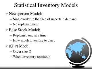
Statistical Inventory Models. Newsperson Model: Single order in the face of uncertain demand No replenishment Base Stock Model: Replenish one at a time How much inventory to carry (Q, r) Model Order size Q When inventory reaches r. Issues. How much to order Newsperson problem

Statistical Inventory Models
E N D
Presentation Transcript
Statistical Inventory Models • Newsperson Model: • Single order in the face of uncertain demand • No replenishment • Base Stock Model: • Replenish one at a time • How much inventory to carry • (Q, r) Model • Order size Q • When inventory reaches r
Issues • How much to order • Newsperson problem • When to order • Variability in demand during lead-time • Variability in lead-time itself
Newsperson Problem • Ordering for a One-time market • Seasonal sales • Special Events • How much do we order? • Order more to increase revenue and reduce lost sales • Order less to avoid additional inventory and unsold goods.
Newsperson Problem Order up to the point that the expected costs and savings for the last item are equal • Costs: Co • cost of item less its salvage value • inventory holding cost (usually small) • Savings: Cs • revenue from the sale • good will gained by not turning away a customer
Newsperson Problem • Expected Savings: • Cs *Prob(d < Q) • Expected Costs: • Co *[1 - Prob(d < Q)] • Find Q so that Prob(d < Q) is Co Cs + Co
Example • Savings: • Cs = $0.25 revenue • Costs: • Co = $0.15 cost • Find Q so that Prob(d < Q) is 0.375 0.15 0.25 + 0.15
Finding Q (An Example) Normal Distribution (Upper Tail) 0 z
Example Continued • If the process is Normal with mean and std. deviation , then (X- )/ is Normal with mean 0 and std. dev. 1 • If in our little example demand is N(100, 10) so = 100 and . • Find z in the N(0, 1) table: z = .32 • Transform to X: (X-100)/10 = .32 X = 103.2
Extensions • Independent, periodic demands • All unfilled orders are backordered • No setup costs Cs = Cost of one unit of backorder one period Co = Cost of one unit of inventory one period
Extensions • Independent, periodic demands • All unfilled orders are lost • No setup costs Cs = Cost of lost sale (unit profit) Co = Cost of one unit of inventory one period
Base Stock Model • Orders placed with each sale • Auto dealership • Sales occur one-at-a-time • Unfilled orders backordered • Known lead time l • No setup cost or limit on order frequency
Different Views • Base Stock Level: R • How much stock to carry • Re-order point: r = R-1 • When to place an order • Safety Stock Level: s • Inventory protection against variability in lead time demand • s = r - Expected Lead-time Demand
Different Tacks • Find the lowest base stock that supports a given customer service level • Find the customer service level a given base stock provides • Find the base stock that minimizes the costs of back-ordering and carrying inventory
Finding the Best Trade-off • As with the newsperson • Cost of carrying last item in inventory = • Savings that item realizes • Cost of carrying last item in inventory • h, the inventory carrying cost $/item/year • Cost of backordering • b, the backorder carrying cost $/item/year
Finding Balance • Cost the last item represents: • h*Fraction of time we carry inventory • h*Probability Lead-time demand is less than R • h*P(X < R) • Savings the last item represents: • b*Fraction of time we carry backorders • b*Probability Lead-time demand exceeds R • b*(1-P(X < R)) • Choose R so that P(X < R) = b/(h + b)
Customer Service Level • What customer service level does base stock R provide? • What fraction of customer orders are filled from stock (not backordered)? • What fraction of our orders arrive before the demand for them? • What’s the probability that lead time demand is smaller than R? • P(X < R)
Smallest Base Stock • What’s the smallest base stock that provides desired customer service level? e.g. 99% fill rate. • What’s the smallest R so that P(X < R) > .99?
Control Policies • Periodic Review • eg, Monthly Inventory Counts • order enough to last till next review + cushion • orders are different sizes, but at regular intervals • Continuous Review • constant monitoring • (Q, R) policy • orders are the same size but at irregular intervals
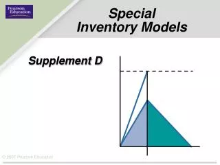
Continuous Review Order Quantity Inventory Reorder Level Safety Stock Time
Safety Stock • Inventory used to protect against variability in Lead-Time Demand Lead-Time Demand: Demand between the time the order to restock is placed and the time it arrives Reorder Point is: R = Average Lead-Time Demand + Safety Stock
Order Quantity • Trade-off • fixed cost of placing/producing order, A • inventory carrying cost, h
A Model • Choose Q and r to minimize sum of • Setup costs • holding costs • backorder costs
Approximating the Costs • Setup Costs • Setup D/Q times per year • Average Inventory is • cycle stock: Q/2 • safety stock: s • Total: Q/2+s • Q/2 + r - Expected Lead-time Demand • Q/2 + r -
Estimating The Costs • Backorder Costs • Number of backorders in a cycle • 0 if lead-time demand < r • x-r if lead-time demand x, exceeds r • n(r) = r(x-r)g(x)dx • Expected backorders per year • n(r)D/Q
The Objective • minimize Total Variable Cost • AD/Q (Setup cost) • h(Q/2 + r - ) (Holding cost) • bn(r)D/Q (Backorder cost)
An Answer • Q = Sqrt(2D(A + bn(r))/h) • P(XŠ r) = 1 - hQ/bD • Compute iteratively: • Initiate: With n(r) = 0, calculate Q • Repeat: • From Q, calculate r • With this r, calculate Q
Another Tack • Set the desired service level and figure the Safety Stock to Support it. • Use trade-off in Inventory and Setups to determine Q (EOQ, EPQ, POQ...)
Variability in Lead-Time Demand • Variability in Lead-Time • Variability in Demand • X = Xt: period t in lead-time) • Var(X) = Var(Xt)E(LT) + Var(LT)E(Xt)2 • s = z*Sqrt(Var(X)) • Choose z to provide desired level of protection.
Safety Stock • Analysis similar to Newsperson problem sets number of stockouts: • Savings of Inventory carrying cost • Cost of One more item short each time we stocked out Co =Stockouts/period*Cs Stockouts/period = Co /Cs
Example • Safety Stock of Raw Material X • Cost of Stocking out? • Lost sales • Unused capacity • Idle workers • Cost of Carrying Inventory • Say, 10% of value or $2.50/unit/year • Number of times to stock out: 2.50/2,500,000 or 1 in a million (exaggerated)
Example • Assuming: • Average Demand is 6,000/qtr (~ 92/day) • Variance in Demand is 100 units2/qtr (1.5/day) • Average Lead Time is 2 weeks (10 days) • Variance in Lead-Time is 4 days2 • Lead-Time Demand is normally distributed • E(X) = 92*10 = 920 • Var(X) = 1.5*10 + 4*(8464) ~ 34,000
Example • Look up 1 in a million on the Normal Upper Tail Chart • z ~ 4.6 • Compute Safety Stock • s = 4.6*Sqrt(34,000) = 4.6*184 = 846 • Compute Reorder Point • r = 920 + 846 = 1,766
Other Issues • Why Carry Inventory? • How to Reduce Inventory? • Where to focus Attention?
Why Carry Inventory? • Buffer Production Rates From: • Seasonal Demand • Seasonal Supplies “Anticipation Inventory”
Other Types of Inventory “Decoupling Inventory” • Allows Processes to Operate Asynchronously • Examples: • DC’s “decouple” our distribution from individual customer orders • Holding tanks “decouple” 20K gal. syrup mixes from 5gal. bag-in-box units.
Other Types of Inventory • “Cycle Stock” • Consequence of Batch Production • Used to Reduce Change Overs: • 8 hours and 400 tons of “red stripe” to change Pulp Mill from Hardwood to Pine Pulp • 4 hours to change part feeders on a Chip Shooter Reduce Setup Time!
Other Types of Inventory “Pipeline Inventory” • Goods in Transit • Work in Process or WIP • Allows Processes to be in Different Places • Example: • Parts made in Mexico, Taurus Assembled in Atlanta
Other Types of Inventory “Safety Stock” • Buffer against Variability in • Demand • Production Process • Supplies • Avoid Stockouts or Shortages
Using Inventory • Inventory Finished Goods or Raw Materials? • Inventory at Central Facility or at DCs? • Extremes: • High Demand, Low Cost Product • Low Demand, High Cost Product
Reducing Inventory • Reducing Anticipation Inventories • Manage Demand with Promotions, etc. • Reduce overall seasonality through product mix • Expand Markets
Reducing Inventory • Reducing Cycle Stock • Reduce the length of Setups • Redesign the Products • Redesign the Process • Move Setups Offline • Fixturing, etc. • Reduce the number of Setups • Narrow Product Mix • Consolidate Production
Reducing Inventory • Reducing Pipeline Inventory • Move the Right Products, eg, Syrup not Coke • Consolidate Production Processes • Redesign Distribution System • Use Faster Modes
Reducing Inventory • Reducing Safety Stock • Reduce Lead-Time • Reduce Variability in Lead-Time • Reduce the Number of Products • Consolidate Inventory
ABC Analysis • Where to focus Attention: Dollar Volume = Unit Price * Annual Demand • Category A: 20% of the Stock Keeping Units (SKU’s) account for 80% of the Dollar Volume • Category C: 50% of the SKU’s with lowest Dollar Volume • Category B: Remaining 30% of the SKU’s