
Statistical Analysis: Gaussian Distribution and Comparisons in Research
E N D
Presentation Transcript
Overview 4-1 Gaussian Distribution 4-2 Comparison on Standard Deviations with the F Test 4-3 Confidence Intervals 4-4 Comparison of Means with Student’s t 4-5 t Tests with a Spreadsheet 4-6 Grubbs Test for an Outlier 4-7 The Method of Least Squares 4-8 Calibration Curves 4-9 A Spreadsheet for Least Squares
4-1: Gaussian Distribution • The results of many measurements of an experimental quantity follow a Gaussian distribution. • The measured mean, x, approaches the true mean, μ,as the number of measurements becomes very large.
4-1: Standard Deviation • The broader the distribution, the greater is s,the standard deviation. • About two-thirds of all • certain interval is proportional to the area of that interval.
4-1: Standard Deviation • For n measurements, an estimate of the standard deviation is • The relative standard deviation expressed as a % is known as the coefficient of variation.
4-1: Standard Deviation and Probability • The mathematical equation for the Gaussian curve is given below. [Equation 4-3] • The maximum occurs for x = μ. . • The probability of observing a value within a certain interval is proportional to the area of that interval. • About two-thirds of all measurements lie within ±1s and 95% lie within ±2s.
4-1: Area Under the Gaussian Distribution • Express deviations from the mean value in multiples, z, of the standard deviation. • Transform x into z, given by: • The probability of measuring z in a certain range is equal to the area of that range. • For example, the probability of observing z between -2 and -1 is 0.136. This probability corresponds to the shaded area in Figure 4-3.
4-1: Standard Deviation of the Mean • The standard deviation s is a measure of the uncertainty of individual measurements. • The standard deviation of the mean, σn is a measure of the uncertainty of the mean of nmeasurements. • Uncertainty decreases by a factor of 2 by making four times as many measurements and by a factor of 10 by making 100 times as many measurements. • Instruments with rapid data acquisition allow us to average many experiments in a short time in order to improve precision.
4-2: Comparing Standard Deviations • The F test is used to decide whether two standard deviations are significantly different from each other. • If Fcalculated ( s12/s22) > Ftable, then the two data sets have less than a 5% chance of coming from distributions with the same population standard deviation.
4-3: Student’s t • Student’s tis a statistical tool. • It is used to find confidence intervals and it is also used to compare mean values measured by different methods. • The Student’s t table is used to look up “t-values” according to degrees of freedom and confidence levels.
4-3: Confidence Intervals • From a limited number of measurements (n), we cannotfind the true population mean, μ, or the true standard deviation, σ. • What we can determine are x and s, the sample mean and the sample standard deviation. • The confidence interval allows us to state, at some level of confidence, a range of values that include the true population mean. t is the student s is the standard deviation is the mean n is the number of trials
4-3: Student’s t • Student’s ttestis also used to compare mean values measured by different methods.
4-3: Hypothesis t Tests • Student’s ttestis also used to compare experimental results. There are three different cases to consider. • Compare mean with μ. • Compare two means and. • Paired data. • Compare same group of samples using two methods. • Different samples! • Samples are not duplicated.
4-3: Hypothesis t Tests Case 1 We measure a quantity several times, obtaining an average value and standard deviation. Does our measured value agree with the accepted value? Case 2 We measure a quantity multiple times by two different methods that give two different answers, each with its own standard deviation. Do the two results agree with each other? Case 3 Sample A is measured once by method 1 and once by method 2; the two measurements do not give exactly the same result. Then a different sample, designated B, is measured once by method 1 and once by method 2. The procedure is repeated for n different samples. Do the two methods agree with each other?
4-4: Using the Student’s t Test • Make a null hypothesis, H0, and an alternate hypothesis, HA. • Null Hypothesis H0 • Difference explained by random error • Alternate Hypothesis HA • Difference cannot be explained by random error • Calculate t • Comparetwith ttableat a given confidence level and degrees of freedom. • If t<ttable, accept the null hypotheses H0. • If t> ttable, reject the null hypotheses H0 and accept HA.
The Equations (1) (2) (3) 4-9b 4-9a or 4-12
Degrees of freedom (equation 4-10b) 4-4: Case 2: Additional Equations Pooled standard deviation spooled (equation 4-9a)
4-4: Example: Case 1 • A coal sample is certified to contain 3.19 wt% sulfur. A new analyticalmethod measures values of 3.29, 3.22, 3.30, and 3.23 wt% sulfur, giving a mean of 3.260and a standard deviation s =0.041. • Does the answer using the new method agree with the known answer? • Calculate the confidence interval for the new method. • If the known answer is not within the calculated 95% confidence interval, then the results do not agree.
4-4: Example: Case1 • Solution: • For n = 4 measurements, there are 3 degrees of freedom and t95%= 3.182 in Table 4-4. • The 95% confidence interval ranges from 3.195 to 3.325 wt%. • The known answer (3.19 wt%) is just outside the 95% confidence interval. • There is less than a 5% chance that new method agrees with the known answer.
Case 1 - Comparison of experimental measurements to a “known” amount
4-4: Student’s t • Student’s t is used to compare mean values measured by different methods. • If the standard deviations are not significantly different (as determined with the F test), find the pooled standard deviation with Equation 4-10 and compute t with Equation 4-9a. • If t is greater than the tabulated value for n1+ n2 -2 degrees of freedom, then the two data sets have less than a 5% chance (p < 0.05) of coming from distributions with the same population mean. • If the standard deviations are significantly different, compute the degrees of freedom with Equation 4-10b and compute t with Equation 4-9b.
4-4: Example: Case 2 (standard deviations similar) • Are 36.14 and 36.20 mM significantly different from each other? Do a t test to find out. The F test indicates that the two standard deviations are not significantly different. Therefore calculate tusing s-pooled.
4-4: Example: Case 3 (paired data) Nitrate concentrations in eight different plant extracts were measured using two different methods (shown in columns A and B) below in Figure 4-8. Is there a significant difference between the methods?
4-4: Example: Case 3 (paired data) • For a given sample, calculate the differences between the methods (column D). Average the differences in order to find and sd(standard deviation). t < ttable, accept the null hypothesis
4-6: Removing outliers The Grubbs test helps you to decide whether or not a questionable datum (outlier) should be discarded. The mass loss from 12 galvanized nails was measured. Mass loss (%): 10.2, 10.8, 11.6, 9.9, 9.4, 7.8, 10.0, 9.2, 11.3, 9.5, 10.6, 11.6; (= 10.16, s = 1.11). Should the value 7.8 be discarded or retained? Because Gcalculated < Gtable, the questionable point should be retained.
4-7: Method of Least Squares • The method of least squares is used to determine the equation of the “best” straight line through experimental data points, yi = mxi + b. We need to find m and b. • Equations 4-16 to 4-18 and 4-20 to 4-22 provide the least-squares slope and intercept and their standard uncertainties.
Find the Best-Fit Line through the Data
In order to make a best fit line, we minimize the magnitude of the deviations (yi -ŷi ) from the line. We want to minimize the total residual error! Because we minimize the squares of the deviations, this is called the method of least squares. ŷi = ycalculated
4-7: Equations for Least-Square Parameters Equation 4-16 Equation 4-17 Equation 4-18
Operation of Determinates D = eh - fg
4-7: Calculating the Uncertainty Equations for estimating the standard uncertainties in y, the slope m, and the intercept b are given below. Equation 4-20 Equation 4-21 Equation 4-22
4-8: Calculating the Uncertainty • Equation 4-27 estimates the standard uncertainty in x from a measured value of y with a calibration curve. • A spreadsheet simplifies least-squares calculations and graphical display of the results. m= slope k= number of replicate measurements for unknown n= number of data points for calibration line = mean of y values in calibration line yc= mean value of measured y for unknown x
4-8: Calibration Curve • A calibration curve shows the response of a chemical analysis to known quantities (standard solutions) of analyte.
4-8: Calibration Curve • When there is a linear response, the corrected analytical signal (signal from sample - signal from blank) is proportional to the quantity of analyte. • The linear range of an analytical method is the range over which response is proportional to concentration. • The dynamic range isthe range over which there is a measurable response to analyte, even if the response is not linear.
4-8: Blank Solutions • Blank solutions are prepared from the same reagents and solvents used to prepare standards and unknowns, but blanks have no intentionally added analyte. • The blank tells us the response of the procedure to impurities or to interfering species in the reagents. • The blank value is subtracted from measured values of standards prior to constructing the calibration curve. • The blank value is subtracted from the response of an unknown prior to computing the quantity of analyte in the unknown.