Chapter 4: Summarizing & Exploring Data (Descriptive Statistics)
Chapter 4: Summarizing & Exploring Data (Descriptive Statistics). Graphics! Graphics! Graphics! (and some numbers). Slides prepared by Elizabeth Newton (MIT) with some slides by Jacqueline Telford (Johns Hopkins University) and Roy Welsch (MIT). Graphical Excellence.

Chapter 4: Summarizing & Exploring Data (Descriptive Statistics)
E N D
Presentation Transcript
Chapter 4: Summarizing & Exploring Data (Descriptive Statistics) Graphics! Graphics! Graphics! (and some numbers) Slides prepared by Elizabeth Newton (MIT) with some slides by Jacqueline Telford (Johns Hopkins University) and Roy Welsch (MIT).
Graphical Excellence • “Complex ideas communicated with • clarity, precision, and efficiency” • Shows the data • Makes you think about substance rather than • method, graphic design, or something else • Many numbers in a small space • Makes large data sets coherent • Encourages the eye to compare different • pieces of the data
Charles Joseph Minard Graphic Depicting Exports of Wine from France (1864) Available at http://www.math.yorku.ca/SCS/Gallery/ Source: Minard, C. J. Carte figurative et approximativedes quantitésde vinfrançais exportés par meren 1864. 1865. ENPC (ÉcoleNationaledes Pontset Chaussées), 1865. Also available in: Tufte, Edward R. The Visual Display of Quantitative Information. Cheshire, CT: Graphics Press, 2001.
Summarizing Categorical Data A frequency table shows the number of occurrences of each category. Relative frequency is the proportion of the total in each category. Bar charts and Pie Charts are used to graph categorical data. A Pareto chart is a bar chart with categories arranged from the highest to lowest (QC:“vital few from the trivial many”). Relative Frequency (%) Spinners Tea Cups Log Drop Water Park Vertical Drop Haunted House Roller Coaster A Roller Coaster B Popularity of attractions at an amusement park
Pie Chart and Bar Chart of Attraction Popularity at an Amusement Park Relative Frequency (%) Relative Frequency (%) Spinners Tea Cups Log Drop Vertical Drop Water Park Roller Coaster A Vertical Drop Roller Coaster B Water Park Haunted House Roller Coaster A Roller Coaster B Tea Cups Spinners Haunted House Log Drop
Charles Joseph Minard Graph showing quantities of meat sent from various regions of France to Paris using pie charts overlaid a map of France (1864) Available at http://www.math.yorku.ca/SCS/Gallery/ Source: Minard, C. J. Carte figurative et approximative des quantités de viande de Boucherie envoyées sur pied par les départments et consommées à Paris. ENPC (École Nationale des Ponts et Chaussées),1858, pp. 44.
Plots for Numerical Univariate Data Scatter plot (vs. observation number) Histogram Stem and Leaf Box Plot (Box and Whiskers) QQ Plot (Normal probability plot)
Scatter Plot of Iris Data observation number This graph was created using S-PLUS(R) Software. S-PLUS(R) is a registered trademark of Insightful Corporation.
Scatter Plot of Iris Data with Observation Number Indicated observation number This graph was created using S-PLUS(R) Software. S-PLUS(R) is a registered trademark of Insightful Corporation.
Plot of data using jitter function in S-Plus observation number observation number This graph was created using S-PLUS(R) Software. S-PLUS(R) is a registered trademark of Insightful Corporation.
Run Chart For time series data, it is often useful to plot the data in time sequence. A run chart graphs the data against time. Frequency Compression Compression Production Order Always Plot Your Data Appropriately -Try Several Ways!
Histogram Data: n=24 Gas Mileage {31,13,20,21,24,25,25,27,28,40,29,30,31,23,31,32,35,28, 36,37,38,40,50,17} Gives a picture of the distribution of data. • Area under the histogram represents sample proportion. Distributions • Use approx. sqrt(n) “bins”- if too many, too jagged; if too few, too smooth (no detail) Miles per gallon • Shows if the distribution is: – Symmetric or skewed – Unimodal or bimodal • Gaps in the data may indicate a problem with the measurement process. Count Axis Note: Bars touch for continuous data, but do NOT touch for discrete data. • Many quality control applications – Are there two processes? – Detection of rework or cheating – Tells if process meets the specifications
Histogram of Iris Data This graph was created using S-PLUS(R) Software. S-PLUS(R) is a registered trademark of Insightful Corporation.
Histogram of Iris Data with Density Curve This graph was created using S-PLUS(R) Software. S-PLUS(R) is a registered trademark of Insightful Corporation.
Stem and Leaf Diagram Cum. Dist. Function Data : Gas Mileage Stem Leaf Count CDF Plot Cum Prob Miles per gallon Shows distribution of data similar to a histogram but preserves the actual data. Can see numerical patterns in the data (like 40’s and 50). Step occurs at each data value (higher for more values at the same data point).
Stem and Leaf Diagram for Iris Data Decimal point is 1 place to the left of the colon This graph was created using S-PLUS(R) Software. S-PLUS(R) is a registered trademark of Insightful Corporation.
Summary Statistics for Numerical Data Measures of Location: Mean ( “average”) : Median: middle of the ordered sample ( like for distribution if Is odd Median if Is even Median of {0,1,2} is 1: n=3 so n+1=4 & (n+1)/2=2 (2ndvalue) Median of {0,1,2,3} is 1.5(assumes data is continuous): n=4 Mode: The most common value
Mean or Median? Appropriate summary of the center of the data? – Mean if the data has a symmetric distribution with light tails (i.e. a relatively small proportion of the observations lie away from the center of the data). – Median if the distribution has heavy tails or is asymmetric. Extreme values that are far removed from the main body of the data are called outliers. – Large influence on the mean but not on the median. Right and left skewness (asymmetry) mode mode (high point) median median mean mean (alphabetic -LEFT skewed) (reverse alphabetic -RIGHT skewed)
Quantiles, Fractiles, Percentiles For a theoretical distribution: The pthquantileis the value of a random variable X, xp, such that P(X<xp)=p. For the normal dist’n: In S-Plus: qnorm(p), 0<p<1, gives the quantile. In S-Plus: pnorm(q) gives the probability. For a sample: The order statistics are the sample values in ascending order. Denoted X(1) ,…X(n) The pth quantileis the data value in the sorted sample, such that a fraction p of the data is less than or equal to that value.
Normal CDF X This graph was created using S-PLUS(R) Software. S-PLUS(R) is a registered trademark of Insightful Corporation.
An algorithm for finding sample quantiles: 1) Arrange observations from smallest to largest. 2) For a given proportion p, compute the sample size × p= np. 3) If npis NOT an integer, round up to the next integer (ceiling (np)) and set the corresponding observation = xp. 4) If np IS an integer k, average the kth and (k + 1)st ordered values. This average is then xp. – Text has a different algorithm
Quantiles, continued (pthquantileis 100pth percentile) • Example: • Data: {0, 1, 2, 3, 4, 5, 6} • = { x(1),x(2),x(3),x(4),x(5),x(6),x(7)} n=7 Q1= ceiling(0.25*7) = 2 ⇒Q1= x (2) = 1 = 25th percentile Q2= ceiling(0.50*7) = 4 ⇒Q2= x (4) = 3 = median (50th percentile) Q3= ceiling(0.75*7) = 6 ⇒Q3= x (6) = 5 = 75th percentile S-Plus gives different answers! Different methods for calculating quantiles.
Measures of Dispersion (Spread, Variability): Two data sets may have the same center and but quite different dispersions around it. Two ways to summarize variability: • Give the values that divide the data into equal parts. • –Median is the 50th percentile • –The 25th, 50th, and 75th percentiles are called • quartiles (Q1,Q2,Q3) and divide the data into four • equal parts. • –The minimum, maximum, and three quartiles are • called the “five number summary” of the data. 2. Compute a single number, e.g., range, interquartile range, variance, and standard deviation.
Measures of Dispersion, continued Range = maximum – minimum Interquartile range (IQR) = Q3 – Q1 Sample variance : Sample standard deviation : Sample mean, variance, and standard deviations are sample analogs of the population mean, variance, and standard deviation (μ, σ2, σ)
Other Measures of Dispersion Sample Average of Absolute Deviations from the Mean: Sample Median of Absolute Deviations from the Median Median of
Computations for Measures of Dispersion • Example: • Data: { 0 , 1 , 2 , 3 , 4 , 5 , 6 } • = { x(1) ,x(2) ,x(3) ,x(4) ,x(5) ,x(6) ,x(7) } mean = (0+1+2+3+4+5+6)/ 7 = 21/ 7 = 3 min = 0, max = 6 Q1= x (2) = 1 = 25th percentile Q2= x (4) = 3 = median (50th percentile) Q3= x (6) = 5 = 75th percentile Range = max -min = 6 -0 = 6 IQR = Q3 -Q1 = 5 -1 = 4 s2= [(02+12+22+32+42+52+62) -7(32)]/(7-1) = [91-63]/6 =4.67 s = sqrt(4.67) = 2.16
Sample Variance and Standard Deviation S2and s should only be used to summarize dispersion with symmetric distributions. For asymmetric distribution, a more detailed breakup of the dispersion must be given in terms of quartiles. For normal data and large samples: – 50% of the data values fall between mean ± 0.67s – 68% of the data values fall between mean ± 1s – 95% of the data values fall between mean ± 2s – 99.7% of the data values fall between mean ± 3s For normally distributed data: IQR=(mean + 0.67s) -(mean -0.67s) = 1.34s
Standard Normal Density X This graph was created using S-PLUS(R) Software. S-PLUS(R) is a registered trademark of Insightful Corporation.
Box (and Whiskers) Plots Visual display of summary of data (more than five numbers) Quantile Box Plot Outlier Box Plot Data : Gas Mileage IQR = Q3 – Q1 Upper Fence = Q3 +1.5 x IQR Lower Fence = Q3 +1.5 x IQR 90th percentile Rectangle: Two lines are called whiskers and extend to the most extreme data values that are still inside the fences. Observations outside the fences are regarded as possible outliers and are denoted by dots and circles or asterisks. median 10th percentile
Box Plot for Iris Data This graph was created using S-PLUS(R) Software. S-PLUS(R) is a registered trademark of Insightful Corporation.
QQ Plots Compare Sample to Theoretical Distribution Order the data. The ith ordered data value is the pth quantile, where p = (i -0.5)/n, 0<p<1. Text uses i/(n+1). (Why can’t we just say i/n)? Obtain quantiles from theoretical distribution corresponding to the values for p. E.g. qnorm(p), in S-Plus for normal distribution. Plot theoretical quantiles vs. empirical quantiles (sorted data). S-Plus: plot(qnorm((1:length(y)-0.5)/n),sort(y)) Fit line through first and third quartiles of each distribution.
QQ (Normal) Plot for Iris Data Quantiles of Standard Normal This graph was created using S-PLUS(R) Software. S-PLUS(R) is a registered trademark of Insightful Corporation.
Normalizing Transformations Data can be non-normal in a number of ways, e.g., the distribution may not be bell shaped or may be heavier tailed than the normal distribution or may not be symmetric. Only the departure from symmetry can be easily corrected by transforming the data. If the distribution is positively skewed, then the right tail needs to be shrunk inward. The most common transformation used for this purpose is the log transformation: x →log x (e.g., decibels, Richter, and Beaufort (?) scales); see Figure 4.11. The square-root transformation provides a weaker shrinking effect; it is frequently used for (Poisson) count data. For negatively skewed data, use the exponential (ex) or squared (x2) transformations.
Normal Probability Plot of data generated from a certain distribution Quantiles of Standard Normal This graph was created using S-PLUS(R) Software. S-PLUS(R) is a registered trademark of Insightful Corporation.
Normal probability plot of log of same data Quantiles of Standard Normal This graph was created using S-PLUS(R) Software. S-PLUS(R) is a registered trademark of Insightful Corporation.
Histogram of the same data X This graph was created using S-PLUS(R) Software. S-PLUS(R) is a registered trademark of Insightful Corporation.
Summarizing Multivariate Data When two or more variables are measured on each sampling unit, the result is multivariate data. If only two variables are measured the result is bivariate data. One variable may be called the x variable and the other the y variable. We can analyze the x and y variable separately with the methods we have learned so far, but these methods would NOT answer questions about the relationship between x and y. –What is the nature of the relationship between x and y (if any)? –How strong is the relationship? –How well can one variable be predicted from the other?
Summarizing Bivariate Categorical Data Two-way Table The numbers in the cells are the frequencies of each possible combination of categories. Cell, row and column percentages can be computed to assess distribution.
Simpson’s Paradox “Lurking variables [excluded from consideration] can change or reverse a relation between two categorical variables!”
Doctors’ Salaries • The interpreter of a survey of doctors’ salaries in 1990 and again in 2000 concluded that their average income actually declined from $97,000 in 1990 to $91,000 in 2000.” • Income is measured here in nominal (not adjusted for inflation) dollars.
What about the “Rest of the Story”? • What deductive piece of logic might clarify the real meaning of this particular pair of statistics? • Look more deeply: Is there a piece missing? • Here is a very simple breakdown of “the numbers” that may help.
Doctors’ Salaries by Age 1980 1990 Age fraction, f1 Income fraction, f2 Income <= 45 0.5 $60,000 0.7 $70,000 >45 0.5 $120,000 0.3 $130,000 Mean $90,000 $88,000
Conclusion • If MD salaries are broken into two categories by age: – Doctors younger than 45 constituted 50% of the MD population in 1980 and 70% in 1990 – Younger doctors tend to earn less than older, more experienced doctors – Parsed by age, MD salaries increased in both age categories!
Gender Bias in Graduate Admissions For this example, see Johnson and Wichern, Business Statistics: Decision Making with Data. Wiley, First Edition, 1997.
Statistical Ideal Randomized study Gender should be randomly assigned to applicants! This would automatically balance out the departmental factor which is not controlled for in the original plaintiff (observational) study. Practical reality Gender cannot be assigned randomly. Control for department factor by comparing admission within department, i.e. controlling for the confounding factor after completion of the study.
“There are lies, damn lies and then there are statistics!” Benjamin Disraeli
Summarizing Bivariate Numerical Data Method 2 Method 1 Is it easier to grasp the relationship in the data between Method A and Method B from the Table or from the Figure (scatter plot)?
Labeled Scatter Plot Year Country Country Country Country Can you see the improvements in the literacy rates for these four countries more easily in the Table or in the Figure? Leterary rate Year
Sample Correlation Coefficient A single numerical summary statistic which measures the strength of a linear relationship between x and y. Where r = covar(x,y)/(stddev(x)*stddev(y)) Properties similar to the population correlation coefficient ρ – Unitless quantity – Takes values between –1 and 1 – The extreme values are attained if and only if the points (xi, yi) fall exactly on a straight line (r = -1 for a line with negative slope and r = +1 for a line with positive slope.) – Takes values close to zero if there is no linear relationship between x and y. •See Figures 4.15, 4.16, 4.17 (a) and (b)