Download
1 / 36
370 likes | 425 Views
Explore the detailed structure of the NICAM model, including horizontal and vertical grid design, parallel processing techniques, and collaboration resources, presented in a virtual lecture by Masaki Satoh from the Univ. of Tokyo. Learn about grid resolution, divergence operators, error reduction strategies, and the concept of "rlevel" for parallelization. Become familiar with the grid indexing methodology and the vertical grid structure in this comprehensive seminar.

E N D
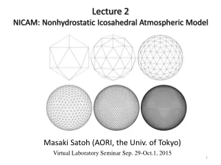
Lecture 2NICAM: Nonhydrostatic Icosahedral Atmospheric Model Masaki Satoh (AORI, the Univ. of Tokyo) Virtual Laboratory Seminar Sep. 29-Oct.1, 2015
contents • Horizontal grid structure • Parallel processing • Vertical grid structure • NICAM collaboration & tutorial code
Discretization of sphere Control volume Hexagon or pentagon Definition of divergence operator
Problem of original icosahedral grid Error of divergence operator (rigid rotation field) Distribution of area of control volume • Large error along the arcs of the original icosahedron • Fractal distribution • Sources of grid noise We expect that smoothing of CV areas will reduce errors.
Modification of icosahedral grid 2. Change of definition point to areal center Second order accuracy • Spring dynamics smoothing mkgrid mkgcgrid
Original icosahedral grid Modified icosahedral grid Tomita, Satoh, Goto (2002,J. Comp. Phys.)
Horizontal uniformity vs b 格子間隔の最大最小比 lmax/ lmin In mkgrid.cnf spr_beta=1.15D0 Standard grid(STD-grid) lmax/lmin 1.34. • Spring grid(SPR-grid) • lmax/lmin: bにも glevelにも依存 • If b =1.2, lmax/lmin 1.24.
Area distributions of control volume Original icosahedral grid Mdified grid Tomita et al. (2001,J. Comp. Phys.)
Parallel strategy (0) rlevel-0 (1) rlevel-1 (2) rlevel-2 (3) rlevel-3
Concept of Horizontal Grid rlevel # of regions 0 10 1 40 2 160 3 640 4 2560 5 10240 • What is “rlevel” ? • Region Division Level • Designed for MPI processes • File name: var-name.rgn????? e.g. sst.rgn00000 ~ sst.rgn00639 • Note: As rlevel increases, total memory consumption is increased, especially when glevel-rlevel is small. • due to halo (overlapped) region. If using 20 processes, 128 regions / process rlevel 1 40 regions / globe rlevel 0 10 regions / globe
Indexing of the horizontal grid • Region structure: diamonds • Structured grid • Fortran 2D array • Efficient for the vector machine • 2d arrays are one-dimensionalized to gain longer vector length. • Vector ratio : more than 99% Typical Arrays V(ij,k,l) Q(ij,k,I,nq)
Prognostic variables ! Prognostic variables ! !--- rho X ( G^{1/2} X gamma2 ) Real(8) :: rhog(ADM_gall_in,ADM_kall,ADM_lall) !--- rho X ( G^{1/2} X gamma2 ) X vx Real(8) :: rhogvx(ADM_gall_in,ADM_kall,ADM_lall) !--- rho X ( G^{1/2} X gamma2 ) X vy Real(8) :: rhogvy(ADM_gall_in,ADM_kall,ADM_lall) !--- rho X ( G^{1/2} X gamma2 ) X vz Real(8) :: rhogvz(ADM_gall_in,ADM_kall,ADM_lall) !--- rho X ( G^{1/2} X gamma2 ) X w Real(8) :: rhogw(ADM_gall_in,ADM_kall,ADM_lall) !--- rho X ( G^{1/2} X gamma2 ) X ein Real(8) :: rhoge(ADM_gall_in,ADM_kall,ADM_lall) !--- rho X ( G^{1/2} X gamma2 ) X eintot Real(8) :: rhogetot(ADM_gall_in,ADM_kall,ADM_lall) !--- rho X ( G^{1/2} X gamma2 ) X q Real(8) :: rhogq(ADM_gall_in,ADM_kall,ADM_lall,TRC_VMAX)
Vertical grid Terrain following coordinate in general form Only the following simplest form is assumed now.
Vertical layer depth: Conversion from real height to model height: Conversion from model height to real height:
NICAM database: horizontal grid data Common data base is prepared: NICAM_DATABASE/hgrid/glxx/rlyy/grid.rgnZZZZZ xx: glevel-xx yy: rlevel-yy ZZZZZ: region id do l_region=1, ADM_lall write (wc(1:5),’(i5.5)’) l_region-1 ! region id ZZZZZ open (fid, file=”grid.rgn”//trim(wc(1:5)), form=”unformatted”, access=”sequential”) read (fid) gall_1d ! Grid number of of one side of region inc. halo (integer) gall = gall_1d*gall_1d ! Total number of region inc. halo (integer) read (fid) GRD_xt (1:gall,1,l_region,GRD_XDIR) ! X-cord. of grid point (real8) read (fid) GRD_xt (1:gall,1,l_region,GRD_YDIR) ! Y-cord. of grid point(real8) read (fid) GRD_xt (1:gall,1,l_region,GRD_ZDIR) ! Z-cord. of grid point (real8) close (fid) end do
Vertical grid data open(fid, file=”vgrid40.dat”, form=”unformatted”, access=”sequential”) read(fid) vlayer ! Total number of vertical layer (integer) kall = vlayer + 2 ! Total number of vertical index inc. top and bottom (integer) allocate ( gz(1:kall) ) allocate ( gzh(1:kall) ) read (fid) gz(:) ! Real height [m] of integer levels (real8) read (fid) gzh(:) ! Real heght [m] of half-integer levels (real8) close (fid)
NICAM collaboration & tutorial code
NICAM development • http://nicam.jp/ • NICAM git server: nicam.jp • Redmine • http://pingpongpearl.aics.riken.jp/redmine/login • NICAM Mail list • admin@nicam.jp: NICAM administrators • M. Satoh, H. Tomita+H. Yashiro+H. Yamaura (AICS), H. Taniguchi(IPRC) • develop@nicam.jp: core developers • contrib@nicam.jp: access to the latest code • users@nicam.jp: access to the tutorial package • All the lecturers are registered to this ML.
Research collaborations • Can use the NICAM code • Can use the NICAM data, especially produced with the Earth Simulator, Athena Project, and K-computer • Can run NICAM on ES or K
TERMS AND CONDITIONS • Do not distribute the NICAM codes to any third party. • Please report any bugs you have found. • Please give us a feedback on the usability of NICAM so as to improve it. • Please let us know the achievements you made with NICAM, so that we can make a list on the NICAM website (http://www.nicam.jp/hiki/?NICAM+Papers) • When you present or publish the results obtained with NICAM, please cite the publications of NICAM. The relevant publications for the NICAM researches can be found in the codes or on the NICAM website. • If a NICAM team member is heavily involved with your project, please acknowledge appropriate members or consider adding him or her as a co-author.
NICAM tutorial package Global NICAM package http://nicam.jp/msn3631/global_nicam/ id: passwd: Regional NICAM package http://nicam.jp/msn3609/reg_nicam/ id: passwd: Common data set http://nicam.jp/msn3609/common_data/ id: passwd:
Temporal scheme • When values at t=A are known, the slow mode tendency S(A) is calculated. • Integrate from A to B using S(A) with fast mode time step. • The slow mode tendency at t=B is calclated: S(B). • Then, integrate from A to C using S(B) with fast mode time step. &TIMEPARAM INTEG_TYPE = 'RK2', LSTEP_MAX = 28800, SSTEP_MAX = 4, DTL = 30.0D0, SPLIT=.TRUE., start_year = 2009, start_month = 7, start_day = 1, / • Slow mode: 2nd order Runge-Kuttaor 3rd order Runge-Kutta • Fast mode: Euler method
Numerical diffusion Horizontal numerical diffusion coefficient KH [m4/s] is forth-order (i.e. KH ∆2 X) Nondimensional diffusion coefficient gamma is defined as KH = gamma dx^4/dt where dx is the grid interval, and dt is the time step. The corresponding diffusion time is tau = dx4/KH = dt/gamma. The empirical rule for the diffusion coefficient: As dx => dx/2, tau => tau/2 This means the diffusion time is proportional to the scale of the meteorological phenomena. Under this condition, if dx => dx/2, dt => dt/2, then gamma should not be changed. In other cases such as dx => dx/2, dt => dt‘, then tau = dt/gamma => tau/2 = dt'/gamma' gamma => gamma' = gamma * ( 2 dt'/dt )
&NUMFILTERPARAM dep_hgrid = .false. lap_order_divdamp = 2, hdiff_type = 'NONLINEAR1', cfact = 2.0D0, Kh_coef_maxlim = 10.0D+16, Kh_coef_minlim = 1.0D+16, ZD_hdiff_nl = 20000D0, divdamp_type = 'DIRECT', alpha_d = 1.0D+16, alpha_dv = 0.00D0, gamma_v = 0.0D0, gamma_h_lap1 = 10.0D+6, ZD_hdiff_lap1 = 20000.0D0, hdiff_fact_rho = 0.01D0, hdiff_fact_q = 0.0d0, ZD = 25000.0d0, alpha_r = 0.0D0, DEEP_EFFECT = .false., /!#### <--- If you increase glevel by one, !#### <--- Kh_coef_maxlim,Kh_coef_minlim, and alpha_d : X(1/8)!#### <--- gamma_h_lap1 : X(1/2) Global model !##--- PARAMETERS for TIME &TIMEPARAM! INTEG_TYPE = 'RK2',! SSTEP_MAX = 4, INTEG_TYPE = 'RK3', SSTEP_MAX = 6, LSTEP_MAX = 720, ! 1hr:10, 1day:240, 2days:480, 3days:720 (if DTL=6min). DTL = 360.0D0, SPLIT = .true., start_year = 2009, start_month = 07, start_day = 01, start_hour = 00, /!#### <--- default : RK2 with SSTEP_MAX = 4;!#### <--- But, if unstable, use RK3 with SSTEP_MAX=6. Glevel 5: dx=220km
!!! GL05/trans_alpha=100/DTL=60sec &NUMFILTERPARAM dep_hgrid = .true., lap_order_divdamp = 2, hdiff_type = 'NONDIM_COEF', gamma_h = 0.0217014, gamma_h_zdep = 0.0325521D0, ZD_hdiff = 20000.0D0, divdamp_type = 'NONDIM_COEF', alpha_d = 0.0217014, alpha_dv = 0.00D0, gamma_v = 0.0D0, gamma_h_lap1 = 0.0D0, ZD_hdiff_lap1 = 20000.0D0, hdiff_fact_rho = 0.01D0, hdiff_fact_q = 1.0d0, ZD = 30000.0d0, alpha_r = 0.0D0, DEEP_EFFECT = .false., / !##### <--- for glevel-9 !#### <--- If glevel-10, Kh_coef_maxlim,Kh_coef_minlim, and alpha_d : X(1/8) !#### <--- gamma_h_lap1 : X(1/2) Stretch model (original) &TIMEPARAM ! INTEG_TYPE = 'RK2', ! SSTEP_MAX = 8, INTEG_TYPE = 'RK3', SSTEP_MAX = 6, LSTEP_MAX = 11520, ! 1day:1440, 2days:2880, 3days: 4230, 7days:10080, @60sec. DTL = 15.0D0, SPLIT = .true., start_year = 2009, start_month = 07, start_day = 01, start_hour = 00, / ! LSTEP_MAX*DTL / 3600 / 24 = 7 (days) !#### <--- default : RK2 with SSTEP_MAX = 4; !#### <--- But, if unstable, use RK3 with SSTEP_MAX=6. Glevel 5: dx_min=22km
Stretch model (present) &NUMFILTERPARAM dep_hgrid = .true., lap_order_divdamp = 2, hdiff_type = 'NONDIM_COEF', gamma_h = 0.0217014, gamma_h_zdep = 0.0325521D0, ZD_hdiff = 20000.0D0, divdamp_type = 'NONDIM_COEF', alpha_d = 0.0217014, alpha_dv = 0.00D0, gamma_v = 0.0D0, gamma_h_lap1 = 0.0D0, ZD_hdiff_lap1 = 20000.0D0, hdiff_fact_rho = 0.01D0, hdiff_fact_q = 1.0d0, ZD = 30000.0d0, alpha_r = 0.0D0, DEEP_EFFECT = .false., / &TIMEPARAM ! INTEG_TYPE = 'RK2', ! SSTEP_MAX = 8, INTEG_TYPE = 'RK3', SSTEP_MAX = 6, LSTEP_MAX = 12, ! 4: 1minute, 240: 1hour, 5760: 1day, @15sec. DTL = 15.0D0, SPLIT = .true., start_year = 2009, start_month = 07, start_day = 01, start_hour = 00, / ! LSTEP_MAX*DTL / 3600 / 24 = 7 (days) !#### <--- default : RK2 with SSTEP_MAX = 4; !#### <--- But, if unstable, use RK3 with SSTEP_MAX=6. Glevel 5: dx_min=22km