Evolution strategies (ES)
450 likes | 653 Views
Evolution strategies (ES). Chapter 4. Evolution strategies. Overview of theoretical aspects Algorithm The general scheme Representation and operators Example Prop er t ies Applications. ES quick overview (I). Developed: Germany in the 1970’s

Evolution strategies (ES)
E N D
Presentation Transcript
Evolution strategies (ES) Chapter 4
Evolution strategies • Overview of theoretical aspects • Algorithm • The general scheme • Representation and operators • Example • Properties • Applications
ES quick overview (I) • Developed: Germany in the 1970’s • Early names: Ingo Rechenberg, Hans-Paul Schwefel and and Peter Bienert (1965), TU Berlin • In the beginning, ESs were not devised to compute minima or maxima of real-valued static functions with fixed numbers of variables and without noise during their evaluation. Rather, they came to the fore as a set of rules for the automatic design and analysis of consecutive experiments with stepwise variable adjustments driving a suitably flexible object / system into its optimal state in spite of environmental noise. • Search strategy • Concurrent, guided by absolute quality of individuals
ES quick overview (II) • Typically applied to: • application concerning shape optimization: a slender 3D body in a wind tunnel flow into a shape with minimal drag per volume. • numerical optimisation; • continuous parameter optimisation • computational fluid dynamics: the design of a 3D convergent-divergent hot water flashing nozzle. • ESs are closer to Larmackian evolution (which states that acquired characteristics can be passed on to offspring). • The difference between GA and ES is the Representation and Survival selection mechanism, that imply survival in the new population of part from the old population
ES quick overview (III) • Attributed features: • fast • good optimizer for real-valued optimisation (real-valued vectors are used to represent individuals) • relatively much theory • Strong emphasis on mutation for creating offspring • Mutation is implemented by adding some random noise drawn from Gaussian distribution • Mutation parameters are changed during a run of the algorithm • In the ES the control parameterare included in the chromosomes and co-evolve with the solutions. • Special: • self-adaptation of (mutation) parameters standard
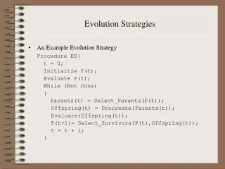
ES Algorithm - The general scheme • An Example Evolution Strategy Procedure ES{ t = 0; Initialize P(t); Evaluate P(t); While (Not Done) { Parents(t) = Select_Parents(P(t)); Offspring(t) = Procreate(Parents(t)); Evaluate(Offspring(t)); P(t+1)= Select_Survivors(P(t),Offspring(t)); t = t + 1; } • The differences between GA and ES consists in representation and survivors selection (in the new population will survive the best of parents and offspring unlike generational genetic algorithms where children replaced the parents).
Evolution Strategies • There are basically 4 types of ESs • The Simple (1+1)-ES (In this strategy the aspect of collective learning in a population is missing. The population is composed of a single individual). • The (+1)-ES (The first multimember ES. parents give birth to 1 offspring) For the next two ESs parents give birth to offspring • The (+)-ES. P(t+1) =Best of the + individuals • The (,)-ES. P(t+1) = Best of the offspring.
(1+1) - Evolution Strategies (two membered Evolution Strategy) • Before the (1+1)-ES there were no more than two rules: • 1. Change all variables at a time, mostly slightly and at random. • 2. If the new set of variables does not diminish the goodness of the device, keep it, otherwise return to the old status. • The Simple (1+1)-ES (In this strategy the aspect of collective learning in a population is missing. The population is composed of a single individual). • (1+1)-ES is a stochastic optimization method having similarities with Simulated Annealing. • Represents a local search strategy that perform the current solution exploitation.
(1+1) - Evolution Strategies features • the convergence velocity, the expected distance traveled into the useful direction per iteration, is inversely proportional to the number of variables of the objective function; • linear convergence order can be achieved if the mutation strength (or mean step-size or standard deviation of each component of the normally distributed mutation vector) is adjusted to the proper order of magnitude, permanently; • the optimal mutation strength corresponds to a certain success probability that is independent of the dimension of the search space and is the range of one fifth for both model functions (sphere model and corridor model). • the convergence (velocity) rate of a ES (1 +1) is defined as the ratio of the Euclidean Distance (ED) traveled towards the optimal point and the number of generations required for running this distance.
Introductory example • Task: minimise f : Rn R • Algorithm: “two-membered ES” using • Vectors from Rn directly as chromosomes • Population size 1 • Only mutation creating one child • Greedy selection
Standard deviation. Normal distribution • Consider X = x1, x2, …,xn n-dimensional random variable. • The mean (μ) M(X)=(x1+ x2,+…+xn)/n. • The square ofstandard deviation (also called variance): 2 = M(X-M(X))2=(xk - M(X))2/n • Normal distribution: N(μ,) = The distribution with μ = 0 and σ2 = 1 is called the standard normal.
Illustration of normal distribution http://fooplot.com/
Introductory example: pseudocode Minimization problem • Set t = 0 • Create initial point xt = x1t,…,xnt • REPEAT UNTIL (TERMIN.COND satisfied) DO • Draw zi from a normal distribution for all i = 1,…,n • yit = xit + zi or yit = xit + N(0, ) • IF f(xt) < f(yt) THEN xt+1 = xt ELSE xt+1 = yt endIF • Set t = t+1 • endDO
Introductory example: mutation mechanism • z values drawn from normal distribution N(μ,) • Mean μ is set to 0 • Standard deviation is called the mutation step size • is varied on the fly by the “1/5 success rule”: • This rule resets after every k iterations by • = / c if Ps > 1/5 (Foot of big hill increase σ) • = • c if Ps < 1/5 (Near the top of the hill decrease σ) • = if Ps = 1/5 • where Psis the % of successful mutations (those in which the child is fitter than parents), 0.8 c 1, usualy c=0.817 • Mutation rule for object variables x (xit) is additive, while the mutation rule for dispersion () is multiplicative.
The Rechenberg’s 1/5th- succes rule • The1/5thrule of success is a mechanism that ensures efficient heuristic search with the price of decreased robustness. • The ratio of successful mutations and other mutations must be the fifth (1/5). • IF this ratio is greater than 1/5 the dispersion must be increased (accelerates convergence). • ELSE • IF this ratio is less than 1/5 the dispersion must be decreased.
The implementation of the Rechenberg’s 1/5th-rule • 1. perform the (1 + 1)-ES for a number G of generations: • − keep σ constant during this period • − count the number Gs of successful mutations during this period • 2. determine an estimate of the success probability Ps by • Ps := Gs/G • 3. change σ according to • σ := σ / c, if Ps > 1/5 • σ := σ · c, if Ps < 1/5 • σ := σ, if Ps = 1/5 • 4. goto 1. The optimal value of the factor c depends on the objective function to be optimized, the dimensionality N of the search space, and on the number G. If N is sufficiently large N ≥ 30, G = N is a reasonable choice. Under this condition Schwefel (1975) recommended using 0.85 ≤ c < 1. Since we are not finding better solutions, we have reached the top of the hill. Rechenberg’s 1/5 rule reduces the standard deviation σ in the case that the system was not very successful in finding better solutions.
Initial shape Final shape Another historical example:the jet nozzle experiment Task: to optimize the shape of a jet nozzle Approach: random mutations to shape + selection
Another historical example:the jet nozzle experiment cont’d In order to be able to vary the length of the nozzle and the position of its throat, gene duplication and gene deletion was mimicked to evolve even the number of variables, i.e., the nozzle diameters at fixed distances. The perhaps optimal, at least unexpectedly good and so far best-known shape of the nozzle was counter-intuitively strange, and it took a while, until the one-component two-phase supersonic flow phenomena far from thermodynamic equilibrium, involved in achieving such good result, were understood.
The disadvantages of (1+1)-ES • Fragile nature of the search point by point based on the 1/5 successful rule may lead to stagnation in a local minimum point. • Dispersion (step size) is the same for each dimension (coordinate) within search space. • Does not use recombination; it is not using a real population • There is no mechanism to allow individual adjustment of stride for each coordinate axis of the search space. The lack of such a mechanism is that the procedure will move slowly to the optimum point.
(+), (,) - (multi membered Evolution Strategies) parents give birth to offspring
Representation • Chromosomes consist of three parts: • Object variables: x1,…,xn • Strategy parameters: • Mutation step sizes: 1,…,n • Rotation angles: 1,…, n • Not every component is always present • Full size: x1,…,xn,1,…,n,1,…, k • where k = n(n-1)/2 (no. of i,j pairs)
Mutation • Main mechanism: changing value by adding random noise drawn from normal distribution • x’i = xi + N(0,) • Key idea: • is part of the chromosome x1,…,xn, • is also mutated into ’ (see later how) • Thus: mutation step size is coevolving with the solution x
Mutate first • Net mutation effect: x, x’, ’ • Order is important: • first ’ (see later how) • then x x’ = x + N(0,’) • Rationale: new x’ ,’ is evaluated twice • Primary: x’ is good if f(x’) is good • Secondary: ’ is good if the x’ it created is good • Reversing mutation order this would not work
Mutation case 1:Uncorrelated mutation with one • Chromosomes: x1,…,xn, • ’ = •exp( • N(0,1)) • x’i = xi + ’• N(0,1) • Typically the “learning rate” 1/ n½ • And we have a boundary rule ’ < 0 ’ = 0
Mutants with equal likelihood Circle: mutants having the same chance to be created
Mutation case 2:Uncorrelated mutation with n ’s • Chromosomes: x1,…,xn, 1,…, n • ’i = i•exp(’ • N(0,1) + • Ni (0,1)) • x’i = xi + ’i• Ni (0,1) • Two learning rate parmeters: • ’ overall learning rate • coordinate wise learning rate • 1/(2 n)½ and 1/(2 n½) ½ • And i’ < 0 i’ = 0
Mutants with equal likelihood Ellipse: mutants having the same chance to be created
Mutation case 3:Correlated mutations • Chromosomes: x1,…,xn, 1,…, n ,1,…, k • where k = n • (n-1)/2 • and the covariance matrix C is defined as: • cii = i2 • cij = 0 if i and j are not correlated • cij = ½•(i2 - j2 ) •tan(2 ij) if i and j are correlated • Note the numbering / indices of the ‘s
Correlated mutations cont’d The mutation mechanism is then: • ’i = i•exp(’ • N(0,1) + • Ni (0,1)) • ’j = j + • N (0,1) • x ’ = x + N(0,C’) • x stands for the vector x1,…,xn • C’ is the covariance matrix C after mutation of the values • 1/(2 n)½ and 1/(2 n½) ½ and 5° • i’ < 0 i’ = 0 and • | ’j | > ’j =’j - 2 sign(’j)
Mutants with equal likelihood Ellipse: mutants having the same chance to be created
Recombination • Creates one child • Acts per variable / position by either • Averaging parental values, or • Selecting one of the parental values • From two or more parents by either: • Using two selected parents to make a child • Selecting two parents for each position anew
Parent selection • Parents are selected by uniform random distribution whenever an operator needs one/some • Thus: ES parent selection is unbiased - every individual has the same probability to be selected • Note that in ES “parent” means a population member (in GA’s: a population member selected to undergo variation)
Survivor selection • Applied after creating children from the parents by mutation and recombination • Deterministically chops off the “bad stuff” • Basis of selection is either: • The set of children only: (,)-selection • The set of parents and children: (+)-selection
Survivor selection cont’d • (+)-selection is an elitist strategy • (,)-selection can “forget” • Often (,)-selection is preferred for: • Better in leaving local optima • Better in following moving optima • Using the + strategy bad values can survive in x, too long if their host x is very fit • Selective pressure in ES is very high ( 7 • is the common setting)
Self-adaptation illustrated • Given a dynamically changing fitness landscape (optimum location shifted every 200 generations) • Self-adaptive ES is able to • follow the optimum and • adjust the mutation step size after every shift !
Self-adaptation illustrated cont’d Changes in the fitness values (left) and the mutation step sizes (right)
Prerequisites for self-adaptation • > 1 to carry different strategies • > to generate offspring surplus • Not “too” strong selection, e.g., 7 • • (,)-selection to get rid of misadapted ‘s • Mixing strategy parameters by (intermediary) recombination on them
ES Applications: • Lens shape optimization required to Light refraction • Distribution of fluid in a blood network • Brachystochrone curve • Solving the Rubik's Cube
Example application: the Ackley function (Bäck et al ’93) • The Ackley function (here used with n =30): • Evolution strategy: • Representation: • -30 < xi < 30 (coincidence of 30’s!) • 30 step sizes • (30,200) selection • Termination : after 200000 fitness evaluations • Results: average best solution is 7.48 • 10 –8 (very good)