Download
1 / 45
450 likes | 499 Views
Explore self-organizing, Hebbian, and error-driven learning in cognitive neuroscience. Learn how topographic representations are created through self-organization, Hebbian correlation learning, and error-driven task learning. Discover the principles of topographical map creation in the brain, including models like SOM (Self-Organized Feature Mapping). Understand the history and key concepts of self-organizing neural networks, competitive learning, and neural plasticity. Dive into the mechanics of SOM algorithm, competition, cooperation, and dynamics in modeling brain plasticity. Gain insights into mapping human body and brain plasticity through the formation of topographical maps. Uncover the role of self-organized networks in cognitive processes.

E N D
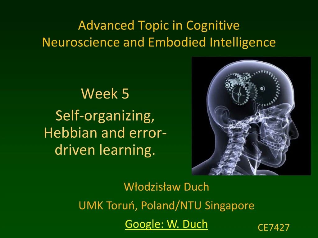
Advanced Topic in Cognitive Neuroscience and Embodied Intelligence Week 5Self-organizing, Hebbian and error-driven learning. CE7427
What it will be about • Self-organized learning: creating topographic representations. • Hebbiancorrelation learning. • Error-driven task learning.
Topographical representations Self-organization is modeled in many ways; simple models are helpful in explaining qualitative features of topographic maps. Many examples, best known are somatosensory and motor primary cortex, but many other motor and sensory areas have topographical organization, including visual and auditory areas. Quantization of perception is useful. How can it arise?
Simplest models Emergent has examples of self-organization of receptive fields in V1 cortex. SOMor SOFM (Self-Organized Feature Mapping) – self-organizing feature map, one of the most popular brain-inspired models. How can topographical maps be created in the brain? Local neural connections create strong groups interacting with each other, weaker across greater distances and inhibiting nearby groups. History: von der Malsburg& Willshaw(1976), competitive learning, Hebbian learning with "Mexican hat" potential, mainly visual system. Amari (1980) – layered models of neural tissue. Kohonen (1981) – simplification without inhibition; left only two essential processes: competition and cooperation. Interaction strength: local cooperation, further inhibition
SOM: idea Data: vectors XT = (X1, ... Xd)from d-dimensional space (samples of signals). Network: nodes with local processors (neurons or columns) in each node. Each local processor # jhas dadaptive parameters W(j). Goal: adjust the W(j)parameters to model clusters in the X space. Sensory data are spatio-temporal, here only rough features of their distribution is determined, this makes it more robust to noise and irrelevant details. Node parameters represent synaptic strength of neurons receiving projections from lower levels (for ex. SI from thalamus); initially they may receive data from random areas, but learning will self-organize overlapping receptive fields.
Training SOM A strip of somatosensory cortex may have neurons reacting to tactile stimuli from different parts of the space, but with sufficient stimulations neurons in the mesh will move their receptive fields (changing their synaptic connections, represented by weight vectors in the model) becoming more sensitive to the areas where real data comes from most often. Creation of topographical maps and modeling of brain plasticity(PPT presentation, 2001, mapping human body).
SOM algorithm: competition Nodes should calculate similarity of input data to their parameters. Input vectorXis compared to the current node parametersW. Similar = minimal distance or maximal scalar product. Competition: find node j=c with W most similar to X. Node number c is most similar to the input vectorX It is a winner of the competition who can handle this input, hence this is a “competitive learning” procedure. According to Hebb rule, the node should learn to be more similar to X. In the brain those neurons that react to some signals will increase their activation in time, learning to analyze this signal in a better way.
SOM algorithm: cooperation Cooperation: nodes on a grid close to the winnercshould behave similarly. Define the “neighborhoodfunction” O(c): t– iteration number (or time); rc – position of the winning node c (in physical space, usually 2D). ||r -rc||– distance from the winning node, scaled by sc(t). e0(t) – slowly decreasing multiplicative factor The neighborhood function determines how strongly the parameters of the winning node and nodes in its neighborhood will be changed, making them more similar to data X.
SOM algorithm: dynamics Adaptation rule: take the winner nodec, and those in its neighborhood O(rc), change their parameters making them more similar to the data X • Randomly select new sample vector X, and repeat. • Decrease h0(t)slowly until there will be no changes. Result: • W(i) ≈the center of local clusters in the X feature space • Nodes in the neighborhood point to adjacent areas in X space
Maps and distortions Initial distortions may slowly disappear or may get frozen if plasticity rapidly decreases ... leaving the brain with a completely distorted view of reality. Most people in the world believe in some conspiracy theories …
Demonstrationsusing GNG Self-Organizing Networksjava GNG demos Many versions of competitive learning implemented in Java. Parameters of the program: t– iterations e(t) = ei (ef/ ei)t/tmaxspecifies a step in learning s(t) = si (sf/ si)t/tmaxspecifies the size of the neighborhood Maps 1x30 show the formation of Peano's curves. An attempt to reconstruct Penfield's maps from responses to touch.
2D => 1D in a triangle The line in the data space forms aPeano curve, an example of a fractal.Why?
What it will be about • Self-organized learning: creating topographic representations. • Hebbian correlation learning. • Error-driven task learning.
Hebbian learning in primary cortex Nagasena-Meander dialogue (100 BC): if it were to rain again, where will this rain water flow? It will flow in the same way as the first water had gone. Electrical current in the brain flows the same way (W. James, 1890). Donald Hebb (1949): Neurons the fire together, wire together. Biological mechanism: synaptic plasticity, or Long Term Potentiation (LTP) and Long Term Depression (LTD). Synchronous stimulation enhances signal transmission between neurons, lasting from minutes to month. Associativity and cooperativity: weak stimulation of several pathways increases LTP effect; strong simulation of one increases other path stimulated weakly. Memory formation (but only spatial memory demonstrated), role in addiction.
Long-Term Potentiation (LTP) was discovered in 1966 first in the hippocampus, then in the cortex. Stimulating a neuron with a current of ~100Hz for 1 second increases synaptic efficiency by 50-100%, and it is a long-term effect. Opposite effect: LTD, Long-Term Depression. Biological foundations: LTP, LTD The most common form of LTP/LTD is related to NMDA (glutamate) receptors. Activity of NMDA channels requires presynaptic as well as postsynaptic activity, in compliance with the Hebb rule. Many other forms of synaptic plasticity exist: short term neural facilitation (paired pulse facilitation) and depression, spike-timing-dependent plasticity (STDP, involves temporal aspects of Hebb rule), and synaptogenesis.
1. Mg2+ ions block NMDA channels. An increase in postsynaptic potential is necessary to remove them and enable interactions with glutamate. 2. Presynaptic activity is necessary to release the glutamate, which opens NMDA channels. 3. Ca2+ ions enter these channels triggering a series of chemical reactions, which are not yet completely understood. NMDA receptors The effect is nonlinear: small amounts of Ca2+ lead to LTD, and large amounts to LTP. Many other processes play a role in LTP.More detailed information on LTP/LTD.
Internal representations of patterns appearing in incoming signals in the environment of a given neural group. Discovering correlations between signals. Model learning positive correlation Elements of images, movements, animal behavior or emotions, we can correlate everything by creating a behavioral model. Only strong correlations are relevant, there are too many weak ones and they can be coincidental. Example: hebb_correl.proj, in Chapter 4.
The two first inputs are completely correlated; the third is uncorrelated. Changes follow according to Hebb's rule for e=1. xi yj=x*w Example Let the signals be zero on average (xi=+1 the same number of times as xi=-1); for each vector x =(x1,x2,x3), y is calculated, and then the new weights. Correlated units determine the symbol and scale of the weights,and weights of these inputs grow quickly, whereas the weight of the uncorrelated input x3decreases. The weights of unit j change in this way: wj(t+1)=wj(t)+Dwj(t)
Select: hebb_correl.proj, in Chapter 4 Click on r.wtin the network window, after clicking on the hidden neuron we see that weights of the entire network have been initialized to 0.5. Simulation Click on act in the network window, on run in the control window In effect we get binary weights => lrate= e =0.005 pright= probability of the first event Defaults changes pright=1 to 0.7
Simple Hebb's rule: Dwij = e xi yj leads to an infinite increase in weights. This can be avoided in many ways; often employed is a normalization of weights: Dwij = e (xi -wij) yj Hebb - normalization This has a biological justification: • when x and y are large we have a strong LTP, much Ca++ • when y is large but x is small we have LTD, some Ca++ • when y is small nothing happens because Mg2+ ions block the NMDA channels.
Hebb's mechanism allows for learning correlations. What happens if we add more postsynaptic neurons? They will learn the same correlations! If we use kWTA then output units will compete with each other. Model learning Learning = survival of the fittest (Darwin's mechanism) + specialization. Learning based on self-organization: • Inhibition of kWTA: only the strongest units remain active. • Hebbian learning: the winners become even stronger. • Result: different neurons react to different signal properties.
Principal component analysis (PCA) is a mathematical technique for finding linear signal combinations with the greatest variance. Standard PCA The first neuron should learn the most important correlations, so first we calculate the correlations of its inputs averaged over time: Cik=xixkt for the first element; then for the next, but each neuron should be independent, so it should calculate orthogonal combinations. For the set of images consecutive components look like this ==> How to do this with the help of neurons?
Let's assume that the environment is composed only of the diagonal lines. Let's accept a linear activation for moment t (image nr t): PCA for one neuron Let the change of weight values be specified by a simple Hebbrule: wij(t+1) = wij(t) + exiyj After presentation of all the images: The change of weights is proportional to the average of the product of the inputs*outputs. Correlation can replace average.
If the averages are zero and the variance is one then the average of the product is the correlation; the change in weights is proportional to: Hebbian Correlations Correlation: Cik=xixktare correlations between inputs; the average of the weights changes slowly. The change in weight for input i is then the weighted average of the correlations between the activity of this input and the remaining ones. After the presentation of many images, the weights will be dominated by the strongest correlations and yjwill calculate the strongest component of PCA.
The simplest normalization avoiding an infinite increase in weights: Dwij = e (xi – wij) yj Erkki Oja (1982) proposed: Dwij = e (xi –yjwij) yj For one unit, after learning the weights stop changing: Dwij = 0 =e (xi –yjwij) yj Weight wij= xi /yj= xi /Skxkwkj The weight of a given input signal is then a fraction of the complete weighted activity of all the signals. This rule also leads to the calculation of the most important main component. How to calculate the other components? Normalization
How to generate the succeeding PCA components in neural networks? We may perform orthogonalization of successive yjnumerically, but this is not easy to do with the help of a neural network. Problems with PCA • Sequential PCA orders components, from the most important to the least; this can be achieved by introducing connections between hidden neurons with strong inhibition, but this is an artificial solution. • PCA assumes a hierarchical structure: the most important component for all images, in effect we get eg. for image analysis, successive components as chessboards with an increasing number of squares since the correlations of pixels for a large number of images disappear. • The problem with PCA can be characterized as: PCA calculates correlations in the entire input space whereas useful correlations exist in local subspaces. • Natural images create heterarchies, different combinations are equally important for different images, subsets of features relevant for certain categories are not important for differentiating others.
Conditional principal component analysis (CPCA): calculate correlations not for all features but only for these features which are present in selected images. Conditional PCA PCA functions on all features, giving orthogonal components. CPCA functions on subsets of features, ensuring that different components encode different interesting combinations of signal features, eg. edges. The competition realized with the help of kWTA will ensure the activity of different neurons for different images. In effect, it will create receptive fields => that can be combined to recreate images How to do this with the help of neurons?
Neurons are trained on subsets of imageswith predetermined features, eg.edges slanting in a certain way.Each subset may be embedded in many uncorrelated patterns, but should be repeated frequently. Normalized Hebb's rule is used: Dwij = e (xi -wij) yj The weights move in direction xi, on condition that there is activity yj. In effect the conditional probability for inputs/outputs in [0,1]: P(xi =1|yj =1) = P(xi|yj) = wij The weight wij = the probability that the input unit xiis active given that the receiving unit yjis also active. For uncorrelated pixels it will be small. CPCA equations
Chapter 4: Self_org.proj, learn in simple environments! Inputs: 5 horizontal and 5 vertical bars, 2 shown at one time: one in some position plus all possible context, all 9*10/2=45 combinations, creating conditional PCA inputs, with correlations for pixels in lines. kWTA, k=2 used. CPCA self-organized learning <= Selective representations appear
The success of CPCA depends on the selection of a function determining the activity of neurons – an automatic determination process is possible in a few ways: self-organization or error correction. Activations averaged over time are represented by probabilities P(xi|t), P(yj|t). The change in weights for all images t appearing with P(t): Dwij = e [St (P(yj|t) P(xi|t)-P(yj|t)wij] P(t) In a state of equilibrium Dwij =0 so: wij = St P(yj|t)P(xi|t)P(t)/ St P(yj|t)P(t) = St P(yj,xi,t)/ St P(yj,t) = P(xi ,yj)/P(yj) = P(xi|yj) Weight wij = conditional probability xiunder condition yj. How to biologically justify normalization? Probabilistic interpretation
Normalized Hebb's rule: Dwij = e (xi -wij) yj Let's assume that the weights are wij ~0.5, there are then 3 possibilities: 1. xi , yj~1 (a strong pre- and postsynaptic activity), so xi > wij, weights increase, so we have LTP, as in NMDA channels. 2. yj~1 but xi < wij, weight decrease, we have LTD, a weak input signal will suffice to unblock the Mg2+ ion of NMDA channel. A strong postsynaptic activity can also unblock other voltage dependent channels and introduce a small amount of Ca++. 3. Activity yj~0 doesn't give any changes, voltage channels and NMDA aren't active. Learning happens faster for small wij, because xi < wijmore often. Qualitatively consistent with observations of weight saturation. Biological interpretation
CPCA weights are not very selective, don't lead to image differentiation – they don't have the dynamic range. For typical situations P(xi|yj) is small, but we want it around 0.5. Solution: renormalization of weights and contrast enhancement. Normalization of weights in CPCA Normalization: uncorrelated signals should have a weight of 0.5, but in simulations with seldom appearing signals xi approach a value of a~0.1-0.2. Let's factorize the weight change into two terms: Dwij = e (xi -wij) yj= e [(1-wij) xiyj+(1-xi)(0-wij)yj] The first term causes an increase in weights in the direction of 1, the second causes a decrease in the direction of 0; if we want to maintain average weights around 0.5 we must increase the first term, eg. : Dwij = e [(0.5/a-wij) xiyj+(1-xi)(0-wij)yj] The linear correlation is still wij= P(xi|yj)0.5/a . The simulator has a parameter savg_cor[0,1] determining the degree of renormalization.
Contrast in CPCA Instead of a linear weight change we want to ignore weak correlations and strengthen strong correlations – to increase the contrast between interesting aspects of signals and those that are not. This increases the simplicity of the connections (the weak ones can be skipped) and accelerates the learning process, helping the weights decide what to do. Contrast enhancement: instead of a linear weight change use a sigmoidal one: Two parameters: gain gand offset q. q>1 imposes higher threshold Attention: this is a scaling of individual weights not of activations!
BCM/XCAL Model More recently BCM rule (Bienenstock, Cooper & Munro, 1982) has been used; assuming homeostatic mechanism that regulate neural activity, each hidden unit should be active for about the same % of time as other units. Dynamic threshold q based on neuron activity is used to modify Hebb rule: Dwij= xi yj(yj-qi), qi = <yj>2 Final neuron output grows for large yand then saturates, similar to the dependence of synaptic plasticity on Ca2+levels. This is effective when: • the relevant features are uniformly distributed in the environment, • there is a good match between the number of units in the hidden layer and the number of features. • Used in the new eXtendedContrastive Attractor Learning (XCAL) model in Emergent, but it is not clear how that changes results.
What it will be about • Self-organized learning: creating topographic representations. • Hebbian correlation learning. • Error-driven task learning.
Hebbian learning based on correlations <xiyj> fails for many mappings X=>Y For example: y=x1.xor.x2, or (0,0)=>0, (1,1)=>0, (0,1)=>1, (1,0)=>1, all <xiyj>=1/2. If y = color green or red, and x = position in 2D correlations are not sufficient. Hebbian learning has problems All two-class categorization problems that are not separable by a single hyperplane cannot be solved this way. For a large number of inputs x almost all problems are not separable. Learning of tasks or general mappings requires another approach.
In task learning there is a goal, and a mechanism to check if it has been reached, so the learning is error-driven. Where do the goals come from? Internal or external teacher: confronting performance with expectations (predictions) of internal models, using burst of dopamine for reward. Input at time t output t+1; ex: speech after reading. Task learning a) explicit input signal, action + correctionsignal; b)internal expectation, action + self-correction; c) implicit motor expectation d) implicit internal reconstruction (internal second input, coming for ex. from parietal cortex).
Delta rule is the optimal way to reduce error in a 2-layer network, without hidden units (Widrow, Hoff 1960), or gradient discent in linear regression. Idea: correctwikweights when errors are large, do not correct where errors are quite small. Delta = error estimation, starting from the output, propagates to input. Delta rule and BP Feedforward step: calculate outputs, backward step: calculate errors and make corrections proportional to these errors.
E(w) – error function depends on all network parameters w, it is an average over all errorsE(X;w)for input patterns X. ok(X;w) – output values of neuron kin the network (y, z values etc) for X. tk(X;w)– target values on kneuron for inputX. For single input X, and one parameterw Error function In minimumE(X;w)for parameterswderivatives are alldE(X;w)/dw = 0. For many parameters derivatives over each parameter are calculateddE/dwi, gradient = 0. Error correction and backpropagation minimization of error f. Errors may not always reach 0, but if the network has sufficiently many parameters for finite number of input patterns X it may find a solution (set of parameters) for which minimum error is reached – but it may lead to overfitting, reducing generalization!
Backpropagation is the most popular approach to mulit-layer perceptron networks but and can learn arbitrary input-output relation, but it is hard to find biological justification for such process. Emergent uses modified rule. GeneRec/XCAL GeneRec (General Recirculation, O’Reilly 1996), Bidirectional flow, wkl wjk, in backprop same weights, and only error flows. Expectation, or minus phase: settle input activations. Hidden units are driven both by inputs and activations that from outputs. Outcome, or plus phase, target values drive the output and hidden units. Plus-minus phase difference approximates BP delta rule Dwij = exi (yj+-yj-)
Both approaches are needed: Hebb + error correction Correlation learning and error terms: - and + phases, expectations and feedbacks, alternate quickly, ~ 0.1 sec. Weighted combination kWTA implements inhibition inside layers, creating sparse internal representations.Neurons compete with each other and only the best neurons, specializing in a given task and only the most confident (i.e. highly active), are left.
Hebbian learning creates a model of basic features of the world, correlations between events and features but is not able to learn heteroasscociations. Hidden layers allow for transformation of data into different feature space while error correction learns arbitrary input-output relations (behaviors). Combined Hebbian correlation learning (xi~yj)and error correction learning should be able to learn everything in a biologically plausible way. Connections in the brain are bidirectional. Combo properties Biology: noCa2+ = no learning; little Ca2+ = LTD, a lot ofCa2+ = LTP. + = LTP, - =LTD in the table, LTD = unfulfilled expectations, only the – phase without enhancement from the + or outcome phase.
Bidirectional connectivity leads to anattractor dynamics, or multiple constraint satisfaction: the network can start off in many initial states (the region called basin of attractor) and evolve towards specific attractor or prototype state, representing cleaned-up, stable interpretation of a noisy or ambiguous input pattern. This state is a compromise between multiple constraints, minimizing overall energy of the system. Multiple constraint satisfaction Color = time, several attractors for words, fast transitions; axis (x,y,x) = position. Color = distance from the point at a given time shown on x, y axis. Attractor dynamics is best visualized using recurrence plots or using Fuzzy Symbolic Dynamics technique to see high-dimensional trajectories.
6 principles embedded in Leabra: integrate & fire point neurons, kWTA, sparse distributed representations, many layers of transformation, Hebb &error correction learning. Leabra learning model Leabra= Learning in an Error-driven and Associative, Biologically Realistic Algorithm So far we are discussing only how local learning is possible, but all this has to be embedded in overall cognitive architecture.