Docking Algorithm Scheme
Enhance docking algorithm schemes through shape representation, patch matching, and transformation filtering. Focus on geometric hashing, steric clash detection, and shape complementarity for accurate candidate scoring.

Docking Algorithm Scheme
E N D
Presentation Transcript
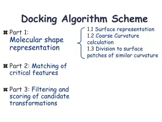
Docking Algorithm Scheme 1.1 Surface representation 1.2 Coarse Curvature calculation 1.3 Division to surface patches of similar curvature • Part 1:Molecular shape representation • Part 2: Matching of critical features • Part 3: Filtering and scoring of candidate transformations
Shape Representation Part • Focus on sparse surface features, preserving the quality of shape representation. • The sparse features reduce the complexity of the matching step.
Docking Algorithm Scheme • Part 1: Molecular shape representation • Part 2:Matching of critical features
Part 2: Matching of patches • The aim is to align knob patches with hole patches, and flat patches with any patch. Two types of matching: • Single Patch Matching – one patch from the receptor is matched with one patch from the ligand. Used in protein-drug cases. • Patch-Pair Matching – two patches from the receptor are matched with two patches from the ligand. Used in protein-protein cases.
Receptor hole patch Ligand knob patch Transformation Single Patch Matching • Base:a pair of critical points with their normals from one patch. • Match every base from a receptor patch with all the bases from complementary ligand patches. • Compute the transformation for each pair of matched bases.
Receptor patches Ligand patches Transformation Patch-Pair Matching • Base:1 critical point with its normal from one patch and 1 critical point with its normal from a neighboring patch. • Match every base from the receptor patches with all the bases from complementary ligand patches. • Compute the transformation for each pair of matched bases.
Base Compatibility • The signature of the base is defined as follows: • Euclidean and geodesic distances between the points: dE, dG • The angles α, β between the [a,b] segment and the normals • The torsion angle ω between the planes dE, dG, α, β, ω Two bases are compatible if their signatures match.
Geometric Hashing • Preprocessing: the bases are built for all ligand patches (single or pairs) and stored in hash table according to base signature. • Recognition: for each receptor base access the hash-table with base signature. The transformations set is computed for all compatible bases. • Clustering: since local features are matched, there may be multiple instances of “almost” the same transformation.
Docking Algorithm Scheme • Part 1: Molecular shape representation • Part 2: Matching of critical features • Part 3:Filtering and scoring of candidate transformations
-1 0 +1 Distance Transform Grid Dense MS surface (Connolly)
Filtering Transformations with Steric Clashes • Since the transformations were computed by local shape features matching they may include unacceptable steric clashes. • Candidate complexes with slight penetrations are retained due to molecular flexibility. • Steric clash test: • For each candidate ligand transformation • transform ligand surface points • For each transformed point • access Distance Transform Grid and check distance value • If it is more than max_penetration • Disqualify transformation
Scoring Shape Complementarity • The scoring is necessary to rank the remaining solutions. • The surface of the receptor is divided into five shells according to the distance function: S1-S5 • [-5.0,-3.6), [-3.6,-2.2), [-2.2, -1.0), [-1.0,1.0), [1.0). • The number of ligand surface points in every shell is counted. • Each shell is given a weight: W1-W5 • -10, -6, -2, 1, 0. • The geometric score is a weighted sum of the number of ligand surface points Ninside every shell: Score=Σ Wip
Filtering and Scoring Performance Problem: the number of surface points for high resolution MS surface may reach 100,000. For each candidate transformation, for each surface point apply the transformation and access distance transform grid. multi-resolution surface data structure supports fast queries for penetrations and geometric score. 16,000 points 1,000 points 119,000 points 4,100 points
Docking Algorithm Scheme The correct solution is found in 90% of the cases with RMSD under 5A. The rank of the correct solution can be in the range of 1 – 1000. • Part 1: Molecular shape representation • Part 2: Matching of critical features • Part 3: Filtering and scoring of candidate transformations WANTED Biochemical Scoring function !!!
Factors that influence the rank of the correct solution • Shape complementarity • Interface shape – in the concave/convex interfaces (enzyme-inhibitor, receptor-drug), shape complementarity is easier to detect comparing to flat interfaces (antibody-antigen). • Sizes of molecules – the larger the molecules the higher the number of the false-positive results.