Random Process
340 likes | 655 Views
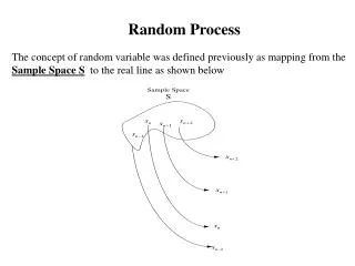
Random Process. The concept of random variable was defined previously as mapping from the Sample Space S to the real line as shown below. The concept of random process can be extended to include time and the outcome will be random functions of time as shown below. The functions.

Random Process
E N D
Presentation Transcript
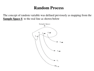
Random Process The concept of random variable was defined previously as mapping from the Sample Space S to the real line as shown below
The concept of random process can be extended to include time and the outcome will be random functions of time as shown below The functions are one realizations of many of the random process X(t) A random process also represents a random variable when time is fixed is a random variable
Stationary and Independence The random process X(t) can be classified as follows: First-order stationary A random process is classified as first-order stationary if its first-order probability density function remains equal regardless of any shift in time to its time origin. If we Xt1let represent a given value at time t1 then we define a first-order stationary as one that satisfies the following equation: The physical significance of this equation is that our density function, is completely independent of t1 and thus any time shift t For first-order stationary the mean is a constant, independent of any time shift
Second-order stationary A random process is classified as second-order stationary if its second-order probability density function does not vary over any time shift applied to both values. In other words, for values Xt1 and Xt2 then we will have the following be equal for an arbitrary time shiftt From this equation we see that the absolute time does not affect our functions, rather it only really depends on the time difference between the two variables.
For a second-order stationary process, we need to look at the autocorrelation function ( will be presented later) to see its most important property. Since we have already stated that a second-order stationary process depends only on the time difference, then all of these types of processes have the following property:
Wide-Sense Stationary (WSS) A process that satisfies the following: is aWide-Sense Stationary (WSS) Second-order stationary Wide-Sense Stationary The converse is not true in general
Time Average and Ergodicity Ergodicity An attribute (سمة )of stochastic systems; generally, a system that tends in probability to a limitingform that is independent of the initial condititions The time average of a quantity is defined as Here A is used to denote time average in a manner analogous to E for the statistical average. The time average is taken over all time because, as applied to random processes, sample functions of processes are presumed to exist for all time.
Let x(t) be a sample of the random process X(t) were the lower case letter imply a sample function (not random function). X(t) the random process x(t) a sample of the random process the random process
Let x(t) be a sample of the random process X(t) were the lower case letter imply a sample function. We define the mean value ( a lowercase letter is used to imply a sample function) and the time autocorrelation function as follows: For any one sample function ( i.e., x(t) ) of the random process X(t), the last two integrals simply produce two numbers. A number for the average and a number for for a specific value of t
Since the sample function x(t) is one out of other samples functions of the random process X(t), The average and the autocorrelation are actually random variables By taking the expected value for and ,we obtain
Correlation Function Autocorrelation Function and Its Properties The autocorrelation function of a random process X(t) is the correlation of two random variables and by the process at times t1 and t2 Assuming a second-order stationary process
Linear System with Random Input In application of random process, the Input-Output relation through a linear system can be described as follows: Here X(t) is a random process and h(t) (Deterministic Function) is the impulse response of the linear system ( Filter or any other Linear System )
Linear System with Random Input Now we can look at input output relation as follows: The Time Domain The output in the time domain is the convolution of the Input random process X(t) and the impulse response h(t), Question: Can you evaluate this convolution integral ? Answer: We can observe that we can not evaluate this convolution integral in general because X(t) is random and there is no mathematical expression for X(t).
The Frequency Domain The output in the Frequency Domain is the Product of the Input Fourier Transform of the input random process X(t) , FX(f) and the Fourier Transform of the impulse response h(t), H(f) the Fourier Transform of the input random process X(t) is a random process the Fourier Transform of the deterministic impulse response the Fourier Transform of the output random process Y(t) is a random process Question : Can you evaluate the Fourier Transform of the input random process X(t) , FX(f) ? Answer: In general no , since the function X(t) in general is random and has no mathematical expression.
Question: How can we describe then the behavior of the input random process and the output random process through a linear time-invariant system ?
as We defined previously the autocorrelation The auto correlation tell us how the random process is varying Is it a slow varying process or a high varying process. Next we will define another function that will help us on looking at the behavior of the random process
Let Sxx(f) ( or Sxx(w)) be the Fourier Transform ofRxx(t) OR OR Since Average Power Then SXX(f) is Power Spectral Density ( PSD ) of the Random Process X(t)
Now let us look at the input-output linear system shown below in the time domain and Frequency domain assuming the Random Process X(t) is WSS Time Domain The Mean of the output, Constant
the mean is constant and the autocorrelationof the output is a function of The Autocorrelation of the output, Y(t) is WSS
