Chapter 1 Random Process
Chapter 1 Random Process. 1.1 Introduction (Physical phenomenon) Deterministic model : No uncertainty about its time- dependent behavior at any instant of time . Random model :The future value is subject to “chance”(probability)

Chapter 1 Random Process
E N D
Presentation Transcript
Chapter 1 Random Process 1.1 Introduction (Physical phenomenon) Deterministic model : No uncertainty about its time- dependent behavior at any instant of time . Random model :The future value is subject to “chance”(probability) Example: Thermal noise , Random data stream 1.2 Mathematical Definition of a Random Process (RP) The properties of RP a. Function of time. b. Random in the sense that before conducting an experiment, not possible to define the waveform. Sample space S function of time, X(t,s) mapping
(1.1) 2T:The total observation interval (1.2) = sample function At t = tk, xj(tk) is a random variable (RV). To simplify the notation , let X(t,s) = X(t) X(t):Random process, an ensemble of time function together with a probability rule. Difference between RV and RP RV: The outcome is mapped into a number RP: The outcome is mapped into a function of time
1.3 Stationary Process Stationary Process : The statistical characterization of a process is independent of the time at which observation of the process is initiated. Nonstationary Process: Not a stationary process (unstable phenomenon ) Consider X(t) which is initiated at t = , X(t1),X(t2)…,X(tk) denote the RV obtained at t1,t2…,tk For the RP to be stationary in the strict sense (strictly stationary) The joint distribution function (1.3) For all time shift t, all k, and all possible choice of t1,t2…,tk
X(t) and Y(t) are jointly strictly stationary if the joint finite-dimensional distribution of and are invariant w.r.t. the origin t = 0. Special cases of Eq.(1.3) 1. for all t and t (1.4) 2. k = 2 , t = -t1 (1.5) which only depends on t2-t1 (time difference)
Figure 1.3 Illustrating the concept of stationarity in Example 1.1.
1.4 Mean, Correlation,and Covariance Function Let X(t) be a strictly stationary RP The mean of X(t) is (1.6) for all t (1.7) fX(t)(x) : the first order pdf. The autocorrelation function of X(t) is for all t1and t2 (1.8)
The autocovariance function (1.10) Which is of function of time difference (t2-t1). We can determine CX(t1,t2) if mX and RX(t2-t1) are known. Note that: 1. mX and RX(t2-t1) only provide a partial description. 2. If mX(t) = mX and RX(t1,t2)=RX(t2-t1), then X(t) is wide-sense stationary (stationary process). 3. The class of strictly stationary processes with finite second-order moments is a subclass of the class of all stationary processes. 4. The first- and second-order moments may not exist.
Properties of the autocorrelation function For convenience of notation , we redefine • The mean-square value 2. 3.
The RX() provides the interdependence information of two random variables obtained from X(t) at times seconds apart
Example 1.2 (1.15) (1.16) (1.17)
We refer to |G(f)| as the magnitude spectrum of the signal g(t), and refer to arg {G(f)} as its phase spectrum.
DIRAC DELTA FUNCTION Strictly speaking, the theory of the Fourier transform is applicable only to time functions that satisfy the Dirichlet conditions. Such functions include energy signals. However, it would be highly desirable to extend this theory in two ways: • To combine the Fourier series and Fourier transform into a unified theory, so that the Fourier series may be treated as a special case of the Fourier transform. • To include power signals (i.e., signals for which the average power is finite) in the list of signals to which we may apply the Fourier transform.
The Dirac delta function or just delta function, denoted by , is defined as having zero amplitude everywhere except at , where it is infinitely large in such a way that it contains unit area under its curve; that is and (A2.3) (A2.4) (A2.5) (A2.6)
Example 1.3 Random Binary Wave / Pulse 1. The pulses are represented by ±Avolts (mean=0). 2. The first complete pulse starts at td. 3. During , the presence of +A or –A is random. 4.When , Tk and Ti are not in the same pulse interval, hence, X(tk) and X(ti) are independent.
4. When , Tk and Ti are not in the same pulse interval, hence, X(tk) and X(ti) are independent.
5. For X(tk) and X(ti) occur in the same pulse interval
6. Similar reason for any other value of tk What is the Fourier Transform of ? Reference : A.Papoulis, Probability, Random Variables and Stochastic Processes, Mc Graw-Hill Inc.
Cross-correlation Function and Note and are not general even functions. The correlation matrix is If X(t) and Y(t) are jointly stationary
Example 1.4 Quadrature-Modulated Process where X(t) is a stationary process and is uniformly distributed over [0, 2]. = 0
1.5 Ergodic Processes Ensemble averages of X(t) are averages “across the process”. Long-term averages (time averages) are averages “along the process ” DC value of X(t) (random variable) If X(t) is stationary,
represents an unbiased estimate of The process X(t) is ergodic in the mean, if The time-averaged autocorrelation function If the following conditions hold, X(t) is ergodic in the autocorrelation functions
1.6Transmission of a random Process Through a LinearTime-Invariant Filter (System) where h(t) is the impulse response of the system If E[X(t)] is finite and system is stable If X(t) is stationary, H(0) :System DC response.
Consider autocorrelation function of Y(t): If is finite and the system is stable, If (stationary) Stationary input, Stationary output
1.7 Power Spectral Density (PSD) Consider the Fourier transform of g(t), Let H(f ) denote the frequency response,
: the magnitude response Define: Power Spectral Density ( Fourier Transform of ) Recall Let be the magnitude response of an ideal narrowband filter Df: Filter Bandwidth (1.40)
Properties of The PSD Einstein-Wiener-Khintahine relations: is more useful than !
Example 1.6 Random Binary Wave (Example 1.3) Define the energy spectral density of a pulse as
Example 1.7 Mixing of a Random Process with a Sinusoidal Process We shift the to the right by , shift it to the left by , add them and divide by 4.
X(t) Y(t) h(t) Relation Among The PSD of The Input and Output Random Processes Recall (1.32) SX (f) SY (f)
Relation Among The PSD and The Magnitude Spectrum of a Sample Function Let x(t) be a sample function of a stationary and ergodic Process X(t). In general, the condition for Fourier transformable is This condition can never be satisfied by any stationary x(t) with infinite duration. We may write If x(t) is a power signal (finite average power) Time-averaged autocorrelation periodogram function
Take inverse Fourier Transform of right side of (1.62) From (1.61),(1.63),we have Note that for any given x(t) periodogram does not converge as Since x(t) is ergodic (1.67) is used to estimate the PSD of x(t)
Example 1.8 X(t) and Y(t) are zero mean stationary processes. Consider Example 1.9 X(t) and Y(t) are jointly stationary.
( g(t): some function) ( e.g g(t): (e) ) 1.8 Gaussian Process Define : Y as a linear functional of X(t) The process X(t) is a Gaussian process if every linear functional of X(t) is a Gaussian random variable Fig. 1.13 Normalized Gaussian distribution
Central Limit Theorem Let Xi , i =1,2,3,….N be (a) statistically independent R.V. and (b) have mean and variance . Since they are independently and identically distributed (i.i.d.) Normalized Xi The Central Limit Theorem The probability distribution of VNapproaches N(0,1) as N approaches infinity.
X(t) Y(t) h(t) Gaussian Gaussian Properties of A Gaussian Process 1.
2. If X(t) is Gaussisan Then X(t1) , X(t2) , X(t3) , …., X(tn) are jointly Gaussian. Let and the set of covariance functions be
3. If a Gaussian process is stationary then it is strictly stationary. (This follows from Property 2) 4. If X(t1),X(t2),…..,X(tn) are uncorrelated as Then they are independent Proof : uncorrelated is also a diagonal matrix (1.85)
1.9 Noise · Shot noise ·Thermal noise k: Boltzmann’s constant = 1.38 x 10⁻²³ joules/K, T is the absolute temperature in degree Kelvin.