Download
1 / 30
310 likes | 386 Views
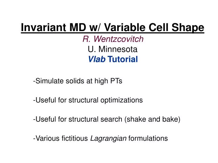
Invariant MD w/ Variable Cell Shape R. Wentzcovitch U. Minnesota Vlab Tutorial. Simulate solids at high PTs Useful for structural optimizations Useful for structural search (shake and bake) Various fictitious Lagrangian formulations. Fictitious molecular dynamics H. C. Andersen (1978).

E N D
Invariant MD w/ Variable Cell ShapeR. WentzcovitchU. MinnesotaVlab Tutorial Simulate solids at high PTs Useful for structural optimizations Useful for structural search (shake and bake) Various fictitious Lagrangian formulations
Fictitious molecular dynamicsH. C. Andersen (1978) (N,H,P) (N,E,V)
Variable Cell Shape MD i=vector index j=cart. index
Anderson’s Fictious MD (HPN ensemble) Anderson’s variable volume fixed shape constant pressure MD (Anderson, J. Chem. Phys 72,2384(1980)) Cell volume The ensemble (trajectory) averages produce the HPN ensemble averages
Fictious MD (continue…) Parrinello/Rahman variable cell shape MD (Parrinello and Rahman, J. Appl. Phys 52, 7182 (1981)) Applying Lagrange’s equation
- in PR-VCSMD is not uniquely defined KLatt a a a a equivalent equivalent The trajectory is not uniquely defined. It does not depend only on the initial conditions.
Solution: use strain ε instead of h as dynamical variable ε is strain Invariant dynamics I Wentzcovitch, PRB 44,2358 (1991)
Alternative form of LInv-I in terms of h and s: with Final observation: In the limit of variable V-only Solution: with Eq. of motion given by Eq. 9 in PRB 44, 2358(1991)
Fluctuations in the cell edges lengths of fcc X-tal of Ar initially placed away from Veq. Beeman integration algorithm dt= 10 fmt (1 a.u. = 2.5 x 10⁻¹⁷s (in Ry)) Mi = 39 mp W= 35 mp in (a); W= 0.0007 mp/ao3 in (b) Rc= 10 ao 2a a a Wentzcovitch, PRB 44,2358 (1991)
fcc Potential energy isosurfaces bcc d sc θ d fcc d Basins of attraction if we use and in the MD fcc bcc bcc sc Basins of attraction if we use and in the PR-MD Wentzcovitch, PRB 44,2358 (1991)
Typical Computational Experiment (Wentzcovitch, Martins, and Price, PRL 1993) Damped dynamics (Wentzcovitch, 1991) P = 150 GPa
hcp to bcc transition in Mg(Wentzcovitch, Phys Rev. B 50, 10358 (1994)) u=1/6 or 1/3 u=1/4 (0001) (110) Atoms at Distortion of the (0001) plane of the hcp structure into the (110) plane of the bcc structure. Arrows indicate atomic displacements.
Enthalpy barrier separating the hcp from the bcc phases at P=35 GPa at T=0K. u=1/6 ↔ hcp u=1/4 ↔ bcc ~150 K Ideal phase boundary (solid) and blurry cause by hysteresis (dashed). Phase transitions will be simulated at the points marked by dots and error bars (undertainties in P and T). Exp. PT = 45-55 GPa at 300 K
u=1/6 u=1/4 u=1/6 u=1/4 hcp to bcc transition Time evolution of the internal parameters u’s, and angles and lengths of simulation cell vectors. Simulation w/ 16 atoms only T = 700 K P = 72 GPa dt = 6 fts W=0.02 mat=24.3 mp u=1/4 Θab = 70.53o Θab = 60o
u=1/6 u=1/4 bcc to hcp transition Time evolution of the internal parameters u’s, and angles and lengths of simulation cell vectors. Simulation w/ 16 atoms only T = 500 K P = 12 GPa dt = 6 fts W=0.02 mat=24.3 mp u=1/6 u=1/4 u=1/4 Θab = 70.53o Θab = 60o
MgSiO3 Perovskite ----- Most abundant constituent in the Earth’s lower mantle ----- Orthorhombic distorted perovskite structure (Pbnm, Z=4) ----- Its stability is important for understanding deep mantle (D” layer)
Pt b c a Crystal structure of post-perovskite Tsuchiya, Tsuchiya, Umemoto, Wentzcovitch, EPSL, 2004 Lattice system: Bace-centered orthorhombic Space group: Cmcm Formula unit [Z]:4 (4) Lattice parameters [Å] a: 2.462 (4.286) [120 GPa] b: 8.053 (4.575) c: 6.108 (6.286) Volume [120 GPa] [Å3]: 121.1 (123.3) ( )…perovskite
Perovskite SiO4 chain SiO3 layer SiO3 Mg SiO3 MgSiO3 Mg SiO3 Ab initio exploration of post-perovskite phase in MgSiO3 - Reasonable polyhedra type and connectivity under ultra high pressure -
θ b’ b c’ Post-perovskite a’ a c Structural relation between Pv and Post-pv Tsuchiya, Tsuchiya, Umemoto, Wentzcovitch, EPSL, 2004 Perovskite Deformation of perovskite under shear strain ε6
Conclusions • VCSMD is very useful for structural optimizations when • the dynamics has the correct symmetry properties • (invariant dynamics) • - It is capable of simulating a phase transition when • one knows how the transformation occurs • - There is unavoidable hysteresis associated with • the simulation, which makes the simulation often • unfeasible • Alternative approaches for obtaining phase boundaries • by computations will be discussed throughout the course
Practice (Go to http://www.msi.umn.edu and navigate to the tutorial web site… …to … software. You will use VCSMD today. Click and download program, Input, and instruction.)
Some Instructions for Lind24-Lab • OpenDX is a visualization software you may use. To enable access to OpenDX: • module load soft/opendx • module initadd soft/opendx • The first line enables the software for the current session, the second for every future session. Every • user will need to type those two lines, but once they do, the software will be permanently enabled for • your individual accounts.To launch the software, type 'dx'. • 2) xmgr is a basic plotting software available in Linux. To launch it type ‘xmgr'. • 3) The command for compiling fortran a code is 'f77'. It's part of the GCC 3.3.5 package built into Linux. • 4) You can SSH to MSI machines. They are on a different network and use a different account, so you • will need to incorporate that into the command. For example, if your username is 'user' and the computer • is 'altix.msi.umn.edu', you would need to type ‘ssh user@altix.msi.umn.edu'. • 5) They machines called lind24-01.itlabs.umn.edu, lind24-02.itlabs.umn.edu, etc, all the way up to • lind24-40.itlabs.umn.edu. Both OpenDX and Xmgr are graphical, so you'll need to enable X Forwarding • for the SSH connection if you're logging in remotely. Usually this can be done by adding the '-XY' flag to • your SSH command in Unix.
Run1 Test: md of Ar atom in fcc cell (title) nd (calc) s n (ic,iio) 11.000000 (alatt) 1 1 1 (nsc) 1.000000 0.000000 0.000000 (avec) 0.000000 1.000000 0.000000 0.000000 0.000000 1.000000 0.00100 0.00000 (cmass, press) 1 (ntype) 4 Ar 40.00000 (natom,nameat,atmass) 0.000000 0.000000 0.000000 (rat) 0.500000 0.500000 0.000000 0.000000 0.500000 0.500000 0.500000 0.000000 0.500000 40.000000 (rcut) 5 5 5 (ncell) 1000 1110 10 (nstep,ntcheck,ntimes) 000.00000 0.00100 200.00000 (temp,ttol,dt) ~
Run2 Decrease step size by ½ and increase # of steps by 2
Run3 Test: md of Ar atom in fcc cell (title) nd (calc) s n (ic,iio) 11.000000 (alatt) 1 1 1 (nsc) 0.500000 0.500000 0.000000 (avec) 0.000000 0.500000 0.500000 0.500000 0.000000 0.500000 0.00100 0.00000 (cmass, press) 1 (ntype) 1 Ar 40.00000 (natom,nameat,atmass) 0.000000 0.000000 0.000000 (rat) 40.000000 (rcut) 9 9 9 (ncell) 2000 2110 10 (nstep,ntcheck,ntimes) 000.00000 0.00100 100.00000 (temp,ttol,dt) ~
Run4 Adjust cell mass to get same period of oscillation
Run5 Test: Optimization under pressure (fcc) (title) nm (calc) s n (ic,iio) 11.000000 (alatt) 1 1 1 (nsc) 1.000000 0.000000 0.000000 (avec) 0.000000 1.000000 0.000000 0.000000 0.000000 1.000000 0.00100 0.00000 (cmass, press) 1 (ntype) 4 Ar 40.00000 (natom,nameat,atmass) 0.000000 0.000000 0.000000 (rat) 0.500000 0.500000 0.000000 0.000000 0.500000 0.500000 0.500000 0.000000 0.500000 40.000000 (rcut) 6 6 6 (ncell) 100 1110 10 (nstep,ntcheck,ntimes) 000.00000 0.00100 500.00000 (temp,ttol,dt) ~
Run6 Test: Optimization under pressure (hcp) (title) nm (calc) s n (ic,iio) 9.000000 (alatt) 1 1 1 (nsc) 1.000000 0.000000 0.000000 (avec) 0.500000 s 0.750000 0.000000 0.000000 0.000000 1.633000 0.00100 0.00000 (cmass, press) 1 (ntype) 2 Ar 40.00000 (natom,nameat,atmass) 0.000000 0.000000 0.000000 (rat) t 1.000000 t 1.000000 0.500000 40.000000 (rcut) 9 9 9 (ncell) 100 1110 10 (nstep,ntcheck,ntimes) 000.00000 0.00100 500.00000 (temp,ttol,dt) ~
Run7 Test: MD of 32 atoms at 200K (title) md (calc) s n (ic,iio) 10.000000 (alatt) 2 2 2 (nsc) 1.000000 0.000000 0.000000 (avec) 0.000000 1.000000 0.000000 0.000000 0.000000 1.000000 0.00100 0.00000 (cmass, press) 1 (ntype) 4 Ar 40.00000 (natom,nameat,atmass) 0.000000 0.000000 0.000000 (rat) 0.500000 0.500000 0.000000 0.000000 0.500000 0.500000 0.500000 0.000000 0.500000 40.000000 (rcut) 3 3 3 (ncell) 1000 100 10 (nstep,ntcheck,ntimes) 200.00000 0.00100 200.00000 (temp,ttol,dt) ~
Run8 Test: MD of 32 atoms at 2000K (title) md (calc) s n (ic,iio) 10.000000 (alatt) 2 2 2 (nsc) 1.000000 0.000000 0.000000 (avec) 0.000000 1.000000 0.000000 0.000000 0.000000 1.000000 0.00100 0.00000 (cmass, press) 1 (ntype) 4 Ar 40.00000 (natom,nameat,atmass) 0.000000 0.000000 0.000000 (rat) 0.500000 0.500000 0.000000 0.000000 0.500000 0.500000 0.500000 0.000000 0.500000 40.000000 (rcut) 3 3 3 (ncell) 1000 100 10 (nstep,ntcheck,ntimes) 2000.00000 0.00100 100.00000 (temp,ttol,dt) ~