Download
1 / 48
480 likes | 705 Views
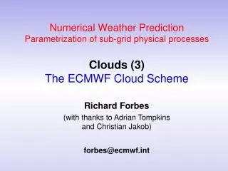
Numerical Weather Prediction Parametrization of sub-grid physical processes Clouds (3) The ECMWF Cloud Scheme. Richard Forbes (with thanks to Adrian Tompkins and Christian Jakob ) forbes@ecmwf.int. The ECMWF Cloud Scheme. Outline. Basic approach Sources and Sinks Convective detrainment

E N D
Numerical Weather Prediction Parametrization of sub-grid physical processesClouds (3)The ECMWF Cloud Scheme Richard Forbes (with thanks to Adrian Tompkins and Christian Jakob) forbes@ecmwf.int
The ECMWF Cloud Scheme Outline • Basic approach • Sources and Sinks • Convective detrainment • Stratiform cloud formation and evaporation • Precipitation generation, melting and evaporation • Ice sedimentation • Ice supersaturation • Summary
ECMWF IFS Cloud Scheme Developments WATER VAPOUR Evaporation Condensation CLOUD FRACTION CLOUD Liquid/Ice Evaporation CLOUD FRACTION Autoconversion PRECIP Rain/Snow Previous Cloud Scheme (operational until 08 Nov 2010) • New Cloud Scheme • (operational from 09 Nov 2010) • Based on Tiedtke (1993) • Prognostic condensate (single moment) & cloud fraction • Diagnostic liquid/ice split as a function of temperature between 0ºC and -23ºC • Diagnostic representation of precipitation • Prognostic liquid & ice & cloud fraction • Prognostic snow and rain (sediments/advects) • Single moment microphysics (mass) • New additional sources and sinks • Existing sources and sink formulation retained (cond/evap/autoconv)
The ECMWF Cloud SchemeBasic assumptions • Clouds fill the whole model layer in the vertical (fraction=cover). • Clouds have the same thermal state as the environmental air (homogeneous T). • Sub-grid variability represented with a cloud fraction prognostic variable and assumptions about the PDF of water vapour and cloud condensate (prognostic statistical cloud scheme). • Considers the physical processes and derives source and sink terms for cloud fraction, ice and liquid cloud condensate and precipitating rain and snow.
y Cloud Cloud free x The ECMWF Cloud SchemeRepresenting sub-grid heterogeneity ECMWF cloud parametrization In the real world y Cloud Cloud free x Humidity variations in cloud-free air but, No in-cloud variability
C G(qt) 1-C qt qs qs The ECMWF Cloud SchemeRepresenting sub-grid heterogeneity ECMWF cloud parametrization In the real world Cloud cover is integral under supersaturated part of PDF G(qt) qt A mixed ‘uniform-delta’ total water distribution is assumed
C G(qt) G(qt) 1-C 1-C C qt qt qs qs The ECMWF Cloud SchemeComparison with Tompkins prognostic PDF scheme Tiedtke(1993) in ECMWF IFS Tompkins (2002) • A mixed ‘uniform-delta’ total water distribution is assumed for the condensation process. • 3 prognostic variables: • Humidity, qv • Cloud condensate, qc • Cloud fraction, C • A bounded beta function with positive skewness. • Effectively 3 prognostic variables: • Mean qt • Variance of PDF • Skewness of PDF Same degrees of freedom ?
3 1 2 4 5 1.Convective Detrainment (deep and shallow) 2. (A)diabatic warming/cooling (radiation/dynamics) 3. Subgrid turbulent mixing (cloud top, horiz eddies) 4. Precipitation generation 5. Precipitation evaporation/melting The ECMWF Cloud SchemeSchematic of sources and sinks Cloud condensate Cloud fraction Some (not all) of these are derived from a pdf approach 6. Advection/sedimentation
The ECMWF Cloud SchemeSources and sinks Cloud liquid water ql(similar for ice) Cloud fraction C Rain qr (similar for snow) A: Transport of Cloud (Advection + Sedimentation) SCV : Detrainment from Convection SBL: Source/Sink Boundary Layer Processes c: Source due to Condensation e/E: Sink due to Evaporation Gp: Precipitation Sink M: Melting
Convective source termLinking clouds and convection Basic idea: Use detrained condensate as a source for cloud water/ice Examples: Ose (1993), Tiedtke(1993), Del Genioet al. (1996), Fowler et al. (1996) Source terms for cloud condensate and fraction can be derived using the mass-flux approach to convection parametrization. Detrainment Subsidence
(-Muql)k-1/2 (-Muql)k+1/2 Convective source termSource of water/ice condensate Vertical advection due to environmental subsidence Detrainment of mass from cumulus updraughts (Muqlu)k-1/2 k-1/2 Standard equation for mass flux convection scheme ECHAM, ECMWF and many others... Duqlu k k+1/2 (Muqlu)k+1/2 Mu= convective updraughtmass flux = environmental subsidence mass flux
(MuC)k-1/2 (MuC)k+1/2 Convective source termSource of cloud fraction Similar equation for the cloud fraction k-1/2 Du k k+1/2
Cloud Condensation and Evaporation Microphysics - ECMWF Seminar on Parametrization 1-4 Sep 2008 14
Convection Cloud formation dealt with separately Turbulent Mixing Cloud formation dealt with separately Stratiform cloud formationChanges in water vapour, q Local criterion for cloud formation: q > qs(T,p) • Two ways to achieve this in an unsaturated parcel: • Increase q • Decrease qs Processes that can increase q in a gridbox Advection
but……… there are numerical problems in models u time, t Stratiform cloud formationNumerical advection Advection does not mix air !!! It merely moves it around conserving its properties, including clouds. qt qs time, t+Dt q2 advection T2 T1 q1 T T1 T2 Because of the non-linearity of qs(T), q2t+Δt> qs(T2 t+Δt) so cloud forms This is a numerical problem and should not be used as cloud producing process! Would be preferable to advect moist conserved quantities instead of T and q
= w(vertical velocity) Stratiform cloud formationChanges in saturation, qs Postulate: The main (but not only) cloud production mechanisms for stratiform clouds are due to changes in qs. Hence we will link stratiform cloud formation to dqs/dt (i.e. changes in p, T).
C G(qt) 1-C qt Stratiform cloud formation: The cloud generation term is split into two components: Existing clouds “New” clouds and assumes a mixed ‘uniform-delta’ total water distribution
Stratiform cloud formation: Increase of existing clouds,c1 C G(qt) qt Already existing clouds are assumed to be at saturation at the grid-mean temperature. Any change in qs will directly lead to condensation. Note that this term would apply to a variety of PDFs for the cloudy air (e.g. uniform distribution)
G(qt) qt Stratiform cloud formation: Formation of new clouds, c2 Due to lack of knowledge concerning the variance of water vapour in the clear sky regions we have to resort to the use of a critical relative humidity, RHcrit G(qt) qt RHcrit = 0.8 is used throughout most of the troposphere
Stratiform cloud formation: Formation of new clouds, c2 For the case of RH>RHcrit We know qe from C G(qt) 1-C qt similarly
Stratiform cloud formation: Formation of new clouds, c2 For the case of RH<RHcrit C G(qt) 1-C Term inactive if RH<RHcrit qt Perhaps for large cooling this is inaccurate? • As stated in the statistical scheme lecture: • With prognostic cloud water and here cover we can write source and sinks consistently with an underlying distribution function • But in overcast or clear sky conditions we have a loss of information. Hence the use of RHcritin clear sky conditions for cloud formation
Evaporation of clouds No effect on cloud cover Processes: e=e1+e2 • Large-scale descent and cumulus-induced subsidence C G(qt) • Diabatic heating qt • Turbulent mixing (e2) Diffusion process proportional to the saturation deficit of the environmental air GCM grid cell Dx where K = 3.10-6s-1 Cloud cover also reduced to keep in-cloud condensate constant
Problem: Reversible Scheme? Cooling: Increases cloud cover C G(qt) 1-C qt Subsequent warming of same magnitude: No effect on cloud cover C G(qt) 1-C qt Process not reversible
Mixed-phase cloud • The previous cloud scheme had a single prognostic variable for cloud condensate. The ice/liquid fraction was diagnosed as a function of temperature between 0°C and -23°C (see dashed line below). • The new cloud scheme has separate prognostic variables for liquid water and ice allowing a wide range of supercooled liquid water for a given temperature (see shading in example below). PDF of liquid water fraction of cloud for the diagnostic mixed phase scheme (dashed line) and the prognostic ice/liquid scheme (shading)
Mixed-phase cloud • The conversion of liquid water to ice is controlled by ice nucleation and ice deposition processes. • Ice nucleation is treated very simply; heterogeneous ice nucleation occurs at temperatures between 0°C and -38°C whenever there is liquid water present (Meyers et al., 1992). • Homogeneous nucleation occurs below -38°C, so no liquid water below -38°C. • If cloud contains water, then assumed to be at water saturation and Bergeron-Findeison mechanism evaporates water and ice grows through deposition: Equation for the rate of change of mass for an ice particle of diameter D due to deposition (diffusional growth), or evaporation • Deposition rate depends primarily on • s = supersaturation • C = particle shape (habit) • F= ventilation factor • Integrate over assumed particles size spectrum to get total ice mass growth
Precipitation Generation + Melting and Evaporation
Gp ql qlcrit Precipitation generationLiquid water clouds Representing autoconversion and accretion in the warm phase. Sundqvist(1978, 1989) Enhancement due to accretion Accretion Gp= autoconversion rate liquid-to-rain P = precipitation rate c1=100 c0=10-4s-1 qlcrit=0.3 g kg-1
Gp ql qlcrit Precipitation generationIce clouds Representing aggregation in the ice phase (conversion ice-to-snow). Rate of conversion of ice (small particles) to snow (large particles) increases as the temperature increases. c0=10-3 e0.025(T - 273.15) s-1 qicrit=3.10-5 kg kg-1
Precipitation melting • The part of the grid box that contains precipitation is • assumed to cool to Tmelt over a timescale tau • Converts snow to rain • Occurs whenever wet bulb temperature Tw > 0°C • Is limited such that cooling does not lead to T<0°C
Precipitation evaporation Cloud Evaporation (Kessler 1969, Monogram) Precip Evap Clear Evap • Evaporation is proportional to the saturation deficit and dependent on the rain mass (g m-3), ρrainclr, in the clear air fraction of the grid box, CPclr. • A diagnostic total precipitation fraction is calculated using a maximum-random overlap treatment of the cloud fraction. • The clear sky fraction is the total precipitation fraction minus the cloud fraction in each layer. • Evaporation reduces the precipitation (implicitly assumes sub-grid precipitation variability).
Clear sky region Grid slowly saturates Precipitation Evaporation Numerical “Limiters” have to be applied to prevent grid scale saturation when precipitation fraction is less than 1 With sub-grid limiter No sub-grid limiter Clear sky region Grid can not saturate
Numerics and sedimentation Advected quantity (e.g. ice) Sedimentation term • Options for sedimentation • (1) semi-Lagrangian • (2) time splitting • (3) implicit numerics Constant Explicit Source/Sink Implicit Source/Sink (not required for shorttimesteps) what is short? Implicit: Upstream forward in time, k = vertical level n = time level f = cloud water (qx) Solution
Ice Sedimentation: Improved numerics in SCM cirrus case • Important to have a sedimentation scheme that is not sensitive to vertical resolution and timestep. Old numerics before CY29R1 Sensitive to vertical resolution Implicit forward-in-time upstream Not sensitive to vertical resolution Vertical profile of ice water content 100 vertical levels (black) versus 50 vertical levels (red)
Cirrus Clouds and Ice Supersaturation Microphysics - ECMWF Seminar on Parametrization 1-4 Sep 2008 36
Air that is supersaturated with respect to ice is common(Pictures courtesy of Klaus Gierens and Peter Spichtinger, DLR) Aircraft flight data 3000 km ice supersaturated segment observed ahead of front Microwave limb sounders
GCM gridbox C Clear sky Cloudy region Cirrus CloudsHomogeneous nucleation • Want to represent super-saturation and homogeneous nucleation • Include simple diagnostic parameterization in existing ECMWF cloud scheme • Desires: • Supersaturated clear-sky states with respect to ice • Existence of ice crystals in locally subsaturated state • Only possible with extra prognostic equation ?
Unlike “parcel” models, or high resolution LES models, we have to deal with subgrid variability GCM gridbox qvenv=? qvcld =? Clear Cloud (qicld) C 1-C We have three items of information: qv, qi, C (grid-box mean vapour, cloud ice and cloud cover) • We know qi occurs in the cloudy part of the gridbox • We know the mean in-cloud cloud ice (qicld=qi/C) • What about the water vapour? In the days of no ice supersaturation: • Clouds: qvcld=qs • Clear sky: qvenv=(qv-Cqs)/(1-C)
In the bad old days No supersaturation 1. (qv-Cqs)/(1-C) qs Lohmann and Karcher: Humidity uniform across gridcell 2. qv qv Klaus Gierens: Humidity in clear sky part equal to the mean total water 3. qv+qi qv-qi(1-C)/C Current assumption including supersaturation: Hang on… Looks familiar??? 4. (qv-Cqs)/(1-C) qs Different approaches to represent clear sky and cloudy humidity GCM gridbox C qvenv qvcld
From Mesoscale Model Lohmann and Karcher: Humidity uniform across gridcell 2. qv qv qvenv qvcld GCM gridbox Critical supersaturationScritreached uplifted box 1 timestep Ice is formed, qi increases, qvcld reduces 1 timestep qvenv=qvcld Artificial flux of vapour from clear sky to cloudy regions!!! Assumption ignores fact that difference processes are occurring on the subgrid-scale
From GCM perspective Current assumption: Hang on… Looks familiar??? 4. (qv-Cqs)/(1-C) qs qvenv qvcld GCM gridbox Critical supersaturationScritreached Difference to standard scheme is that environmental humidity must exceed Scrit to form new cloud (rather than just exceeding ice saturation) uplifted box qvcld reduces to qs qvenv unchanged qi increases microphysics qidecreases qvenv unchanged No artificial flux of vapour from clear sky to cloudy regions Assumption seems reasonable: BUT! Does not allow nucleation or sublimation timescales to be represented, due to hard adjustment to ice saturation in the cloud
Ice supersaturation and homogeneous nucleation • What is Scrit ? • Classical theory and laboratory experiments document the critical vapour saturation mixing ratio with respect to ice at which homogeneous nucleation initiates from aqueous solution drops (Pruppacher and Klett, 1997; Koop et al., 2000). • Leads to supersaturated RH threshold as a function of temperature (Koop et al., 2000, Kärcher and Lohmann, 2002).
Ice supersaturation and homogeneous nucleation Evolution of an air parcel subjected to adiabatic cooling at low temperatures Scrit Evolution of an air parcel subjected to adiabatic cooling at low temperatures Dotted line: Evolution if ice supersaturation is allowed until reaches Scrit Dotted line: Evolution if no ice supersaturationallowed From Tompkins et al. (2007) adapted from Kärcher and Lohmann (2002)
B C A RH wrt ice PDFat 250hPaone month average Aircraft observations A: Numerics and interpolation for default model B: The RH=1 microphysics mode C: Drop due to GCM assumption of subgrid fluctuations in total water
Summary of ECMWF Scheme • Scheme introduces prognostic equations for cloud fraction, cloud liquid water, cloud ice, rain and snow. • Sources and sinks for each physical process. • Some derived using assumptions concerning subgrid-scale PDF for vapour and clouds. J More simple to implement than prognostic variance/skewness in a statistical PDF scheme. Also nicer for assimilation since prognostic quantities directly observable. L Loss of information (no memory) in clear sky (a=0) or overcast conditions (a=1) (critical relative humidities necessary etc). • Nothing to stop solution diverging for cloud cover and cloud water. (eg. ql>0, a=0). Unphysical “safety switches” necessary. • Artificial split between prognostic ice and diagnostic snow variables. • Many microphysical assumptions are empirically based.
Next time: Cloud Scheme Validation….. • Observations, • Observations, • Observations !
References Jakob, C., and S. A. Klein, 2000: A parametrization of the effects of cloud and precipitation overlap for use in general-circulation models. Quart. J. Roy. Meteorol. Soc., 126, 2525-2544. Sundqvist, H. Berge, E., Kristjansson, J. E., 1989: Condensation and cloud parametrization studies with a mesoscale numerical weather prediction model. Mon. Wea. Rev., 177, 1641-1657. Tiedtke, M. 1993: Representation of clouds in large scale models. Mon. Wea. Rev., 117, 1779-1800. Tompkins, A. M., K. Gierens and G. Radel, 2007: Ice supersaturation in the ECMWF integrated forecast system. Quart. J. Roy. Meteorol. Soc., 133, 53-63.