NUMERICAL WEATHER PREDICTION ( Data Assimilation Part)

1. NUMERICAL WEATHER PREDICTION (Data Assimilation Part) Dr Meral Demirtaş Turkish State Meteorological Service Weather Forecasting Department WMO, Training Course, 26-30 September 2011 Alanya, Turkey

2. Outline • Introduction • Basic concepts • Observation resources • Data assimilation techniques

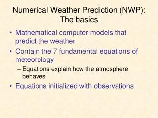
3. Introduction • NWP is an initial/boundary value problem. • • Having the following conditions, the model simulates or forecasts the evolution of the atmosphere. • – an estimate of the present state of the atmosphere • (initial conditions) • – suitable surface and lateral boundary conditions • • The more accurate the estimate of the initial conditions, the better the quality of the forecasts. • • Operational NWP centres produce initial conditions through a statistical combination of observations and short-range forecasts. This approach is called data assimilation.

4. The purpose of a data assimilation is to blend in observations originating from different sources with information contained in a prior estimate of the state of the atmosphere (background). The background is modified to incorporate new observations by combining new and old information in a statistically optimal way. Then, the role of an NWP model is to carry the information gained from past observations forward in time.

5. Data Assimilation (DA) Processes • Ingesting the data • Decoding coded observations • Weeding out bad data • Comparing the data to first guess fields • Interpolating the data on to the model grid for making the forecast

6. Observational data pre-processing Preliminary work: • Check out duplicate reports • Hydrostatic check • Black-listing: Data skipped due to systematic bad performance • Thinning:Some data are not fully used to avoid over-sampling and correlated errors Quality control (QC) • First guess based rejections • Variational QC rejections Compute increments Analysis

8. Aircraft: Wind, Temperature SYNOP/METAR/SHIP: MSLP,10m-u/v, 2m-rh. Pilot/Profilers: Wind TEMP: Wind, T, q

9. DRIBU: MSL Pressure, Wind-10m

10. Remote sensing retrievals • Atmospheric Motion Vectors (AMV) (geo/polar). • SATEM thickness. • Ground-based GPS Total Precipitable Water • SSM/I oceanic surface wind speed and TPW. • Scatterometer oceanic surface winds. • Radar radial velocity and reflectivity • Satellite temperature/humidity/thickness profiles. • GPS refractivity (e.g. COSMIC). • HIRS: NOAA-16, NOAA-17, NOAA-18, METOP-2 • AMSU-A: NOAA-15, NOAA-16, NOAA-18, • AMSU-B: NOAA-15, NOAA-16, NOAA-17 • AIRS: EOS-Aqua • SSMIS: DMSP-16 • EOS-Aqua, METOP-2

14. Data coverage issues • Primitive equation based models have a number of degrees of freedom in the order of 107. • For a time window of +/-3 hours, there are typically10 to 100 thousand observations of the atmosphere. They are distributed non-uniformly in space and time. It is necessary to use additional information, called the background field, first guess or prior information. • A short-range forecast is used as the first guess in operational data assimilation practices. • Current operational systems typically use a 3/6-h cycle performed four times a day.

15. In the operational NWP practice, it is not sufficient to perform spatial interpolation of observations into regular grids. There are not enough data available to define the initial state. The number of degrees of freedom in an NWP model is of the order of 107, while the total number of conventional observations is of the order of 104–105. • Therearemany newtypesofdatasuchas satellite andradar observations, but: • they do not directlymeasurethevariables usedinthemodels • theirdistributioninspaceandtimeis verynon-uniform.

16. In addition to observations, it is necessary to use a first guess estimate of the state of the atmosphere at the grid points. • The first guess (or background field) is our best estimate of the state of the atmosphere prior to the use of the observations. • A short-range forecast is normally used as a first guess in operational systems in what is called an analysis cycle. • Over data rich regions, the analysis is dominated by the information contained in the observations. • In data-poor regions, the forecast benefits from the information coming from the upstream. • For instance, 6-h forecasts over the North Atlantic Ocean are usually good, because of the information coming from the observation rich North America. The model is able to transport information from data-rich to data-poor areas.

17. Globalanalysiscycle. Regionalanalysiscycle.

18. Data Assimilation (DA) Techniques • Empirical Assimilation Methods • Successive Corrections-Iterative analysis (empirical) • Newtonian Relaxation (nudging) • Sequential Methods • Optimal interpolation (OI) (statistical) • 3-Dimentional “VARiational” DA (statistical) • Non-Sequential Methods • 4-Dimentional “VARiational” DA (statistical) • Ensemble Kalman Filter (advanced) • Hybrid methods: • Combinations of ensemble DA techniques: ETKF-3DVar, EnKF-4DVar (advanced)

19. Recalling Some Basics of Statistics • Supposewehavethepressure, piandtemperature, Ti,everydayforayear.Let n=365. • The meanpressure is: • and like-wise formeantemperature. • The variance ofpressure: • and like-wise fortemperaturevariance σ2T . • The standarddeviations, σpand σT arethesquarerootsof thevariances.Theymeasurethe rootmeansquaredeviation fromthemean.

20. The covariance of p and T is defined as: • The correlation between p and T is the normalized covariance: • It is a dimensionless number, and bound between -1 and +1. • If p and T tend to be greater than their mean values at the same time, or less than their mean values at the same time, they are positively correlated and ρpT > 0. • If p tends to be greater than its mean value when T is less than its mean, and vice-versa, then p and T are negatively correlated and ρpT < 0.

21. Fundementals of a DA System • An assimilation system deals with: • Observations (yo) • Background field (xb) • Observation and forecast errors and statistics • An assimilation system generates an analysis (synthesis). Analysis is used in a number of avenues: • Initial conditions for NWP models • Climatology and re-analyses • Observing system design

22. Say the back ground field is a model 6-h forecast: xb If the observed quantities are not the same as the model variables, the model variables are converted to observed variables: yo The first guess of the observations is denoted as: H(xb) where H is the observation operator. The difference between the observations and the background: yo − H(xb) It is referred as the observational increment or innovation.

23. A schematic illustration of innovation vectors The difference between observations and the first guess are taken at the observation location and referred as innovation vectors(yo-H(x)). Observations (yo) First guess at the grid points (Xb) First guess at the observation location H(Xb) The innovation vector (yo-H(Xb))

24. The analysis xa is obtained by adding the innovations to the background field with weights W that are determined based on the estimated statistical error covariances of the forecast and the observations: xa = xb +W[yo − H(xb)] Different analysis schemes (SCM, OI, 3D-Var,and KF) are based on this equation, but differ by the approach taken to combine the background and the observations to produce the analysis. Earlier methods such as the SCM used weights which were determined empirically.The weights were a function of the distance between the observation and the grid point, and the analysis was iterated several times.

25. In Optimal Interpolation (OI), the matrix of weights W is determined from the minimization of the analysis errors at each grid point. • In the 3D-Var approach, one defines a cost function proportional to the square of the distance between the analysis and both the background and the observations. This cost function is minimized to obtain the analysis. • Lorenc (1986) showed that OI and the 3D-Var approach are equivalent if the costfunction is defined as: The cost function J measures: • The distance of a field x to the observations (first term) • The distance to the background xb (second term).

26. The distances are scaled by the observation error covariance R and by the background error covariance B respectively. The minimum of the cost function is obtained for x=xa, which is defined as the analysis. • The analysis obtained by OI and 3D-Var is the same if the weight matrix is given by • W=BHT(HBHT+R−1)−1 • The difference between OI and the 3D-Var approach is in the method of solution: • • In OI, the weights W are obtained for each grid point or • grid volume, using suitable simplifications. • • In 3D-Var, the minimization of J is performed directly, allowing for additional flexibility and a simultaneous global use of the data.

27. The variational approach has been extended to four dimensions, by including within the cost function the distance to observations over a time interval (assimilation window). This is called four-dimensional variational assimilation (4DVar). • In the analysis cycle, the importance of the model may be stressed as: • • It transports information from data-rich to data-poor regions. • • It provides a complete estimation of the four-dimensional state of the atmosphere.

28. Variational Data Assimilation Formulation • Invariationalassimilation,weminimizea costfunction, J,whichisnormallyasumoftwoterms: JBis the distance between the analysis and the background field JO isthedistancetotheobservations:

29. A Schematic illustration of variational DA

30. 3D-Var minimization cost function Jb Jo • Where: • x: model state variable (dimension N) • xb: background field • B: background-error covariance matrix • H: forward interpolation (linear or non-linear) • y: observation vector for the observations • R: observation-error covariance matrix Inpractice, thesolutionisobtainedthrough minimizationalgorithms for J(x)usingiterativemethodsforminimization; the conjugategradient or quasi-Newton methods.

31. A schematic representation of the cost function in a simple 1-D case.

32. Uncertainties in the initial state: Ensembles Initial state Ensemble mean Ensemble members observed (idealized!) Ensemble members time

33. Why do we need a hybrid DA system? • A 3D-VAR system uses only climatological (static) background error covariances. • Flow-dependent covariance through ensemble is needed. • Hybrid combines climatological and flow-dependentbackground error covariances. • It can be adapted to an existing 3D-VAR system. • Hybrid can be robust for small size ensembles.

34. Ensemble Formulation Basics • Assume the following ensemble forecasts: • Ensemble mean: • Ensemble perturbations: • Ensemble perturbations in vector form:

35. The Hybrid Formulation… Ensemble covariance is implemented into the 3D-VAR cost function via extendedcontrol variables: Conserving total variance requires: C: correlation matrix for ensemble covariance localization Weighting coefficient for static 3D-VAR covariance 3D-VAR increment Total increment including hybrid Weighting coefficient for ensemble covariance Extended control variable

36. A hybrid (3DVAR –ETKF) system design and implementation WRF Ensemble: M1 M2 M3 M4 M5 …. Mn Compute: Ensemble perturbations (ep2): u,v,t,ps,q, mean, and std_dev WRF-VAR (hybrid) Update:ensemble mean Compute: ensemble mean WRF-VAR (QC-OBS): filtered_ob.ascii WRF deterministic forecast run WRF-VAR (VERIFY): ob.etkf ensemble ETKF:Update ens perturbations WRF ensemble run for the next cycle Update: ens. initial conditions cycling Update: ens. boundary conditions (Demirtas et al. 2009)

37. Data Assimilation Problems • Transferring information from the scattered locations and times of the observations to the model grid, while the same time. • Preserving the inter-related physical, dynamical and numericalconsistency in the short-range forecast, since these are essential for making consistently good NWP forecasts.

38. Acknowledgements: • Thanks to documents/images of ECMWF, P. Lynch (UoD) and various others that provided excellent starting point • for this talk!

39. Thanks for attending….