Download
1 / 40
400 likes | 418 Views
Cube-based atmospheric GCMs at CSIRO: reversible staggering. John McGregor CSIRO Marine and Atmospheric Research Aspendale, Melbourne MetOffice, Exeter 24 October 2012 Acknowledgements: Marcus Thatcher and Martin Dix. Outline. CCAM formulation VCAM formulation Some comparisons Plans

E N D
Cube-based atmospheric GCMs at CSIRO: reversible staggering John McGregor CSIRO Marine and Atmospheric Research Aspendale, Melbourne MetOffice, Exeter 24 October 2012 Acknowledgements: Marcus Thatcher and Martin Dix
Outline • CCAM formulation • VCAM formulation • Some comparisons • Plans • At Newton Institute • Sorted out VCAM advection • Solved “grid imprinting” problem • Cured 2-grid-point convection noise
Major problem in dynamical cores is how to provide suitable velocity components for the Coriolis terms, so as to give good geostrophic adjustment. The approach in CCAM and VCAM is based on “reversible staggering” of velocity components.
Alternative cubic grids OriginalSadourny (1972) C20 grid Equi-angular C20 grid Conformal-cubicC20 grid
CCAM is formulated on the conformal-cubic grid Orthogonal Isotropic The conformal-cubic atmospheric model Example of quasi-uniform C48 grid with resolution about 200 km
atmospheric GCM with variable resolution (using the Schmidt transformation) 2-time level semi-Lagrangian, semi-implicit total-variation-diminishing vertical advection reversible staggering - produces good dispersion properties a posteriori conservation of mass and moisture CCAM dynamics CCAM physics • cumulus convection: • - mass-flux scheme, including downdrafts, entrainment, detrainment • - up to 3 simultaneous plumes permitted • includes advection of liquid and ice cloud-water • - used to derive the interactive cloud distributions (Rotstayn 1997) • stability-dependent boundary layer with non-local vertical mixing • vegetation/canopy scheme (Kowalczyk et al. TR32 1994) • - 6 layers for soil temperatures • - 6 layers for soil moisture (Richard's equation) • enhanced vertical mixing of cloudy air • GFDL parameterization for long and short wave radiation
Location of variables in grid cells All variables are located at the centres of quadrilateral grid cells. However, during semi-implicit/gravity-wave calculations, u and v are transformed reversibly to the indicated C-grid locations. Produces same excellent dispersion properties as spectral method (see McGregor, MWR, 2006), but avoids any problems of Gibbs’ phenomena. 2-grid waves preserved. Gives relatively lively winds, and good wind spectra.
Where U is the unstaggered velocity component and u is the staggered value, define (Vandermonde formula) accurate at the pivot points for up to 4th order polynomials solved iteratively, or by cyclic tridiagonal solver excellent dispersion properties for gravity waves, as shown for the linearized shallow-water equations Reversible staggering | X | X * | X |m-1 m-1/2 m m+1/2 m+1 m+3/2 m+2m+3/4
Dispersion behaviour for linearized shallow-water equations Typical atmosphere case - large radius deformation Typical ocean case - small radius deformation N.B. the asymmetry of the R grid response disappears by alternating the reversing direction each time step, giving the same response as Z (vorticity/divergence) grid
Pressure advection equation Define an associated variable, similar to MSLP which varies smoothly, even over terrain. It is thus suitable for evaluation by bi-cubic interpolation, whilst the other term is found “exactly” by bi-linear interpolation (to avoid any overshooting effects). Formally, get Treatment of psadvection near terrain
Similarly to surface pressure advection, define an associated variable which varies relatively smoothly on sigma surfaces over terrain. Again the second term can be found “exactly” by bi-linear interpolation. A suitable function is Formally, get This technique effectively avoids the requirement for hybrid coordinates. Treatment of T advection near terrain
Helmholtz solver By suitable manipulation, the SLSI leads to a set of Helmholtz equations for each of the vertical modes, on a 5-point stencil. The Helmholtz equations may be solved by simple successive over-relaxation. A vectorized solution is achieved by solving successively on each of the following 3 sets of sub-grids. A conjugate-gradient solver is also available, and is usually used. 3-colour scheme used for SOR solution of Helmholtz equations (conformal octagon grid has 4-colour scheme)
MPI implementation Remapped region 0 Original Remapping of off-processor neighbour indices to buffer region Indirect addressing is used extensively in CCAM - simplifies coding
Typical MPI performance • Showing both Face-Centred and Uniform decompositionfor global C192 50 km runs, for 1, 6, 12, 24, 48, 72, 96, 144, 192, 288 CPUs (strong scaling example) • VCAM slightly slower, but is still to be fully optimised
Tuning/selecting physics options: In CCAM, usually done with 200 km AMIP runs, especially paying attention to Australian monsoon, Asian monsoon, Amazon region No special tuning for stretched runs An AMIP run 1979-1995 DJF JJA Obs CCAM
Variable-resolution conformal-cubic grid • The C-C grid is moved to locate panel 1 over the region of interest • The Schmidt (1975) transformation is applied • this is a pole-symmetric dilatation, calculated using spherical polar coordinates centred on panel 1 • it preserves the orthogonality and isotropy of the grid • same primitive equations, but with modified values of map factor • Plot shows a C48 grid (Schmidt factor = 0.3) with resolution about 60 km over Australia
Schmidt transformation can be used to obtain even finer resolution Grid configurations used to support Alinghi in America’s Cup Also Olympic sailing for Beijing and Weymouth (200 m) C48 8 km grid over New Zealand C48 1 km grid over New Zealand
Downscaled forecasts 60 km When running the 8 km simulation, a digital filter is used to diagnose large-scale and fine-scale fields. The large-scale fields are then inherited every 3 hours from the 60 km run. 8 km 1 km
Being a semi-Lagrangian model, CCAM is able to absorb the extra phi terms into its Helmholtz equation solver, for “zero” cost The new dynamical core (VCAM) uses a split-explicit treatment, so the Miller-White treatment would need its own Helmholtz solver, so may need another treatment for VCAM Miller-White nonhydrostatic treatment
CCAM simulations of cold bubble, 500 m L35 resolution, on highly stretched global grid
Gnomonic grid showing orientation of the contravariant wind components Illustrates the excellent suitability of the gnomonic grid for reversible interpolation – thanks to smooth changes of orientation
uses equi-angular gnomonic-cubic grid - provides extremely uniform resolution - less issues for resolution-dependent parameterizations reversible staggering transforms the contravariant winds to the edge positions needed for calculating divergence and gravity-wave terms flux-conserving form of equations preferred for trace gas studies TVD advection can preserve sharp gradients forward-backward solver for gravity waves (split explicit) avoids need for Helmholtz solver linearizing assumptions avoided in gravity-wave terms New dynamical core for VCAM - Variable Cubic Atmospheric Model
Horizontal advection Low-order and high-order fluxes combined using (lively) Superbee limiter Cartesian components (U,V,W) of horizontal wind are advected Flow=qyVj+1/2 vcov (qx,qy) q ucov Ui-1/2 Flow=qxUi+1/2 Vj-1/2 Transverse components (included in both low/high order fluxes) calculated at the centre of the grid cells (loosely following LeVeque)
Eastwards solid body rotation in 900 time steps Using superbee limiter Problem caused by spurious vertical velocities at vertices!
Improved treatment of pivot points at panel edges | X | X* | X |m-1 m-1/2 m m+1/2 m+1 m+3/2 m+2m+3/4 edge Usual pivot velocity (in terms of staggered u) is um+3/4= (um+1/2+um+3/2)/2 In terms of unstaggered U, it is Um+3/4= (2Um+6Um+1)/8 But adjacent to panel edge it is better to use Um+3/4 = (-Um-1 + 3Um + 7Um+1 - Um+2)/8 which is derived by using an estimate for Um+1/2 provided by averaging 1-sided extrapolations of U. These extrapolations will be very accurate for velocities such as solid body rotation
Reduction of “grid imprinting” Spurious vertical velocities reduced by factor of 8 by improved calculation of pivot velocities near panel edges
With better staggered velocities at panel edges (avoiding the spurious vertical velocities)
Solution procedure • Start tloop • Nx(Dt/N) forward-backward loop • Stagger (u, v) t+n(Dt/N) • Average ps to (psu, psv) t+n(Dt/N) • Calc (div, sdot, omega) t+n(Dt/N) • Calc (ps, T) t+(n+1)(Dt/N) • Calc phi and staggered pressure gradient terms, then unstagger these • Including Coriolis terms, calc unstaggered (u, v) t+(n+1)(Dt/N) • End Nx(Dt/N) loop • Perform TVD advection (of T, qg, Cartesian_wind_components) using average ps*u, ps*v, sdot from the N substeps • Calculate physics contributions • End t loop • Main MPI overhead is the reversible staggering at each substep, but this just needs nearest neighbours in its iterative tridiagonal solver. • Message passing is also needed in the pressure gradient and divergence calcs
500 hPa omega (avg. Jan 1979) Hybrid coordinates introduced Non-hybrid
Example of effect on rainfall of hybrid coordinates Non-hybrid coords Hybrid coords 32
Avoidance of 2-grid rainfall over Indonesia Small Indonesian islands provide convective forcing at 2-grid length scale – was a persistent feature. Problem solved by spreading the convective heating over the forward-backward time steps.
Absence of noise problems • Some groups report noise problems with split-explicit methods, requiring diffusive suppression methods • No divergence damping or other noise suppression is needed in VCAM, thanks to • - use of reversible staggering (N.B. significant noise is seen if simple interpolation of velocity components is used in Coriolis terms) • - hybrid coordinates • - application of convective heating over the forward-backward time steps
CCAM VCAM 250 hPa windsin a 1-year run- similar
Same physics DJF JJA Obs Climate (rainfall & MSLP) VCAM 1-year CCAM 1-year
VCAM advantages No Helmholtz equation needed Includes full gravity-wave terms (no T linearization needed) Mass and moisture conserving More modular and code is “simpler” No semi-Lagrangian resonance issues near steep mountains Simpler MPI (“computation on demand” not needed) VCAM disadvantages Restricted to Courant number of 1, but OK since grid is very uniform Some overhead from extra reversible staggering during sub time-steps (needed for Coriolis terms) Nonhydrostatic treatment will be more expensive Comparisons of VCAM and CCAM
Tentative conclusions • Reversible staggering works well for both CCAM and VCAM • VCAM seems to perform better than CCAM in the tropics • better rain over SPCZ and Indonesia • possibly by avoiding linearizing ps term in pressure gradients, and better gravity wave adjustment by not using semi-implicit • rainfall needs improving over China
CABLE canopy/carbon scheme has been included mixed-layer-ocean available aerosol scheme added urban scheme added TKE boundary scheme available new GFDL radiation scheme available new version on gnomonic grid (VCAM), in flux-conserving form (being able to achieve conservation is another advantage of stretched global models) – now working coupling to PCOM (parallel cubic ocean model) of Motohiko Tsugawa from JAMSTEC - underway (3:way: CSIRO + JAMSTEC + CSIR_SouthAfrica) Model developments Equi-angular gnomonic C20 grid