Space-Time Data Modeling A Review of Some Prospects

Space-Time Data ModelingA Review of Some Prospects Upmanu Lall Columbia University

Irregularly recorded water quality data form an Attribute Series • A point feature class defines the spatial framework • Many variables defined at each point • Time of measurement is irregular • May be derived from a Laboratory Information Management System Field samples Laboratory Database

Fecal Coliform in Galveston Bay(Irregularly measured data, 1995-2001) Coliform Units per 100 ml Tracking Analyst Demo

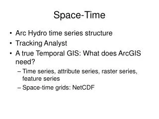
Nexrad over South Florida • Real-time radar rainfall data calibrated to raingages • Received each 15 minutes • 2 km grid • Stored by SFWMD in Arc Hydro time series format

Time series from gages in Kissimmee Flood Plain • 21 gages measuring water surface elevation • Data telemetered to central site using SCADA system • Edited and compiled daily stage data stored in corporate time series database called dbHydro • Each time series for each gage in dbHydro has a unique dbkey (e.g. ahrty, tyghj, ecdfw, ….)

Domain of Applications • Given Space-time data on one or more variables: • Forecast or conditionally simulate process at unobserved space-time locations • One variable conditional on others or on s-t index • Multivariate field • Arbitrary process model or related to physics • Smooth or filter data to recover process • Interpret residuals as “noise” or high or low frequency space-time correlated random field that may relate to covariates • Aggregate-disaggregate process in space and/or time • Clustering, classification, fusion, mining, risk assessment, insurance, data assimilation • Build on same basic ideas, but ……lives to fight another day

Key Concepts and Building Blocks • Linear Model • Generalized Linear Model • Generalized Least Squares • Generalized Additive Model –Nonlinear, Nonparametric • Mixture Models • Multi-Resolution/Frequency Domain Models • Random Fields • State Space Models • Bayesian Models • Hierarchical Bayesian Models  Recommended Framework

Generalized Linear Model Two major changes 1.yiassumed to come from any member of the exponential family, e.g., Binomial, Gamma, Poisson, Gumbel…. 2. Link Function (transformed mean is linear in predictors) Generalized Least Squares Allow noise process to be spatially or temporally correlated e.g., e~N(0,S), where S is a covariance matrix Then Recursive Max. Likelihood Solution Example: y is rain or no rain – Binomial Link function: logistic reg. Example: Serially Correlated Errors (AR1) and X={1} Linear Model y= Xb+e e~N(0,s2); X = {1, t, sin(wt), log(t), loess(t)} yi~N(mi, s2) mi=xib e.g., TREND MODEL with uncorrelated errors Likelihood Models

Summary For space-time, spatial or time series models, we can consider a common general framework: • Datai = Trend (meani) + correlated noisei • Data may correspond to a non-normal model, including mixtures of exponential family members (GLM) • meani can depend nonlinearly on space or time index or covariates • Correlated noise can be modeled as a time series process, or using variograms; space and time correlations are possible (GLS) • Typically stationary noise processes are considered, but mixtures can be used to build nonstationary models • Spatial correlation functions can be parametric or nonparametric • If meani is a constant, and the noise process is weakly stationary (correlation depends only on lag or separation), then • for time data, we have a traditional time series model, • for spatial processes, the ordinary Kriging model, and • for space-time data we could have a markov random field model • GLS+GLM=Likelihood Models  a nice and obvious segway to Bayesian Estimation

The setting • Data Z(s,t) at multiple, irregularly sampled spatial locations s at certain times t • Sampling in space usually irregular and sparse, but could be on a grid, and data may represent changing support • Z(.,.) may be multivariate: represent a vector of variables at each sampling point, or the same variable at a point and/or an areal value (multi-resolution) • Time is ordered, but space is not. Space may be continuous, time may be continuous or discrete • Cases to consider: • Fixed spatial locations, all sampled at the same time – forecast or conditionally simulate process at other times • Can estimate space and time covariance matrices for this set • Space and time sampling locations vary

Mean function can depend on s, t and covariates as before GLM For data irregularly sampled in time, a “variogram” like idea can be used to compute correlations – define and evaluate form and parameters

Example – Spatial Time Series • We have N locations and T times at which we wish to model process: all locations have data at fixed time (missing values allowed) • State Space Model/Dynamic Linear Model Data: Z(s,t) Process: Y(s,t) Measurement Equation: Zt= FtYt + et et~N(0,St), St= N*N spatial covariance State Equation: Yt= GtYt-1+ ntnt~N(0,Snt), Snt = P*P spatial covariance Zt = N*T data matrix Yt=P*T state space Ft= N*P Observation to State map Gt= P*P matrix These two matrices are allowed to change with time nonstationary model Gt could be lag 1 auto and cross-correlations  lot of parameters!! Ft could be Identity if P=N, else it can be used to map obs sites to grid averages

An example of a space-time model that follows from this formulation is: The data Z(s,t) is modeled as a space-time mean field + measurement or high frequency noise The mean process is related to a set of covariates or predictors (can be s, t) The “regression” coefficient of this mean function is modeled as a spatially averaged random walk process with correlation across predictors (b) spatially varying random walk perturbation in the coefficients with correlation across perturbation in b and scale control

How can we estimate a reliable model that has so many parameters and structure? • Need a lot of data • Recognize that there is a lot of shared information in space-time data sets • Model structure allows exploration of spatial and temporal means and effects – mean can be separable also • Bayesian and Hierarchical Bayesian Models for Inference

From C. Wikle w/o permission

State Equation The H matrix is now a tridiagonal matrix  dramatic reduction in the number of parameters from assuming a spatial neighborhood model From C. Wikle w/o permission

X = space-time data matrix on habitat covariates, e.g., human population, temperature, precipitation, land use So, diffusion coefficient can be spatially and temporally variable conditional on predictors Can build similar relations for growth etc From C. Wikle w/o permission

u Log(l) From C. Wikle w/o permission

References • Banerjee, S., B. R. Carlin, A. E. Gelfand, Hierarchical Modeling and Analysis for Spatial Data, Chapman and Hall, 2004 • Gelman, A., et al, Bayesian Data Analysis, Chapman and Hall, 2004 • Anselin, L., Space-Time Models, http://sal.agecon.uiuc.edu • Gelfand, A. E., On the change of support problem for space-time data, Biostatistics, 2001, 2(1), P. 31-45 • Kyriakidis, P.C., and A.G. Journel, Geostatistical Space–Time Models: A Review, Mathematical Geology, 1999, 31(6), 651-684 • Cesare, L. D., D. Meyers, D. Posa, Estimating and modeling space-time correlation structures, Statistics & Probability Letters, 2001, 51, 9-14. • Wikle, C.K., L. M. Berliner, N. Cressie, Hierarchical Bayesian space-time models, Env. And Ecological Statistics, 1998, 5, 117-154 • Wikle, C.K., Ralph F. Milliff, Doug Nychka, and L. Mark Berliner, Spatiotemporal Hierarchical Bayesian Modeling: Tropical Ocean Surface Winds, JASA, 2001, 96(454), 382-397 • Huang, H-C, G. Johannesson and N. Cressie, Multi-Resolution Spatio-Temporal Modeling, http://www.stat.sinica.edu.tw/hchuang

Space-Time Data Modeling A Review of Some Prospects