Decision Tree
Decision Tree. By Wang Rui State Key Lab of CAD&CG 2004-03-17. Review. Concept learning Induce Boolean function from a sample of positive/negative training examples. Concept learning can be cast as Searching through predefined hypotheses space Searching Algorithm: FIND-S

Decision Tree
E N D
Presentation Transcript
Decision Tree By Wang Rui State Key Lab of CAD&CG 2004-03-17
Review • Concept learning • Induce Boolean function from a sample of positive/negative training examples. • Concept learning can be cast as Searching through predefined hypotheses space • Searching Algorithm: • FIND-S • LIST-THEN-ELIMINATE • CANDIDATE-ELIMINATION
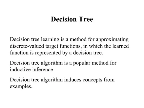
Decision Tree Decision tree learning is a method for approximating discrete-valued target functions(Classifier), in which the learned function is represented by a decision tree. Decision tree algorithm induces concepts from examples. Decision tree algorithm is a general-to-specific searching strategy Examples Decision tree algorithm Decision Tree concept New example classification
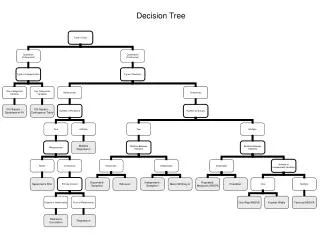
Decision Tree Representation Classify instances by sorting them down the tree from the root to some leaf node • Each branch corresponds to attribute value • Each leaf node assigns a classification
Each path from the tree root to a leaf corresponds to a conjunction of attribute tests (Overlook = Sunny) ^ (Humidity = Normal) • The tree itself corresponds to a disjunction of these conjunctions (Overlook = Sunny ^ Humidity = Normal) V (Outlook = Overcast) V (Outlook = Rain ^Wind = Weak)
Top-Down Induction of Decision Trees Main loop: 1. A the “best” decision attribute for next node 2. Assign A as decision attribute for node 3. For each value of A, create new descendant of node 4. Sort training examples to leaf nodes 5. If training examples perfectly classified, Then STOP, Else iterate over new leaf nodes
{ Outlook = Sunny, Temperature = Hot, Humidity = High, Wind = Strong } • Tests attributes along the tree • typically, equality test (e.g., “Wind=Strong”) • other tests (such as inequality) are possible
Which Attribute is Best? • Occam’s razor: (year 1320) • Prefer the simplest hypothesis that fits the data. • Why? • It’s a philosophical problem. • Philosophers and others have debated this question for centuries, and the debate remains unresolved to this day.
Shorter trees are preferred over lager Trees Idea: want attributes that classifies examples well. The best attribute is selected. How well an attribute alone classifies the training data? information theory Simple is beauty
Information theory • A branch of mathematics founded by Claude Shannon in the 1940s. • What is it? • A method for quantifying the flow of information across tasks of varying complexity • What is information? • The amount our uncertainty is reduced given new knowledge
Information Measurement • Information Measurement • The amount of information about an event is closely related to its probability of occurrence. • Units of information: bits • Messages containing knowledge of a low probability of occurrence convey relatively large amount of information. • Messages containing knowledge of high probability of occurrence convey relatively little information.
Information Source • Source alphabet of n symbols {S1, S2,S3,…Sn} • Let the probability of producing be for • Question • A. If a receiver receives the symbol in a message, how much information is received? • B. If a receiver receives in a M - symbols message, how much information is received on average?
Question A The information of a single symbol in a n symbols message Case I: Answer: is transmitted for sure. Therefore, no information. Case II: Answer: Consider a symbol ,then the received information is So the amount of information or information content in the symbols is
Question B • The information is received on average Message will occur, on average, times for Therefore, total information of the M-symbol message is The average information per symbol is and Entropy
Entropy in Classification • A collection S, containing positive and negative examples, the entropy to this boolean classification is • Generally
Information Gain • What is the uncertainty removed by splitting on the value of A? • The information gain of S relative to attribute A is the expected reduction in entropy caused by knowing the value of A • : the set of examples in S where attribute A has value v
A1 = overcast: + (4.0) A1 = sunny: | A3 = high: - (3.0) | A3 = normal: + (2.0) A1 = rain: | A4 = weak: + (3.0) | A4 = strong: - (2.0) See/C 5.0
Issues in Decision Tree • Overfit • Hypothesis overfitsthe training data if there is an alternative hypothesis such that • h has smaller error than h’ over the training examples, but • h’ has a smaller error than h over the entire distribution of instances
Solution • Stop growing the tree earlier Not successful in practice • Post-prune the tree • Reduced Error Pruning • Rule Post Pruning • Implementation • Partition the available (training) data into two sets • Training set: used to form the learned hypothesis • Validation set : used to estimate the accuracy of this hypothesis over subsequent data
Pruning • Reduced Error Pruning • Nodes are removed if the resulting pruned tree performs no worse than the original over the validation set. • Rule Post Pruning • Convert tree to set of rules. • Prune each rules by improving its estimated accuracy • Sort rules by accuracy
Continuous-Valued Attributes • Dynamically defining new discrete-valued attributes that partition the continuous attribute value into a discrete set of intervals. • Alternative Measures for Selecting Attributes • Based on some measure other than information gain. • Training Data with Missing Attribute Values • Assign a probability to the unknown attribute value. • Handling Attributes with Differing Costs • Replacing the information gain measure by other measures or
Boosting: Combining Classifiers The most material of this part come from:http://sifaka.cs.uiuc.edu/taotao/stat/chap10.ppt By Wang Rui
Boosting • INTUITION • Combining Predictions of an ensemble is more accurate than a single classifier • Reasons • Easy to find quite correct “rules of thumb” however hard to find single highly accurate prediction rule. • If the training examples are few and the hypothesis space is large then there are several equally accurate classifiers. • Hypothesis space does not contain the true function, but it has several good approximations. • Exhaustive global search in the hypothesis space is expensive so we can combine the predictions of several locally accurate classifiers.
Cross Validation • k-fold Cross Validation • Divide the data set into k sub samples • Use k-1 sub samples as the training data and one sub sample as the test data. • Repeat the second step by choosing different sub samples as the testing set. • Leave one out Cross validation • Used when the training data set is small. • Learn several classifiers each one with one data sample left out • The final prediction is the aggregate of the predictions of the individual classifiers.
Bagging • Generate a random sample from training set • Repeat this sampling procedure, getting a sequence of K independent training sets • A corresponding sequence of classifiers C1,C2,…,Ck is constructed for each of these training sets, by using the same classification algorithm • To classify an unknown sample X, let each classifier predict. • The Bagged Classifier C* then combines the predictions of the individual classifiers to generate the final outcome. (sometimes combination is simple voting)
Boosting • The final prediction is a combination of the prediction of several predictors. • Differences between Boosting and previous methods? • Its iterative. • Boosting: Successive classifiers depends upon its predecessors. Previous methods : Individual classifiers were independent. • Training Examples may have unequal weights. • Look at errors from previous classifier step to decide how to focus on next iteration over data • Set weights to focus more on ‘hard’ examples. (the ones on which we committed mistakes in the previous iterations)
Boosting(Algorithm) • W(x) is the distribution of weights over the N training points ∑ W(xi)=1 • Initially assign uniform weights W0(x) = 1/N for all x, step k=0 • At each iteration k: • Find best weak classifier Ck(x) using weights Wk(x) • With error rate εk and based on a loss function: • weight αk the classifier Ck‘s weight in the final hypothesis • For each xi , update weights based on εk to get Wk+1(xi ) • CFINAL(x) =sign [ ∑ αi Ci (x) ]
AdaBoost(Algorithm) • W(x) is the distribution of weights over the N training points ∑ W(xi)=1 • Initially assign uniform weights W0(x) = 1/Nfor all x. • At each iteration k: • Find best weak classifier Ck(x) using weights Wk(x) • Compute εk the error rate as εk= [ ∑ W(xi )∙ I(yi ≠ Ck(xi )) ] / [ ∑ W(xi )] • weight αk the classifier Ck‘s weight in the final hypothesis Set αk = log ((1 –εk )/εk ) • For each xi , Wk+1(xi ) = Wk(xi ) ∙ exp[αk ∙ I(yi ≠ Ck(xi ))] • CFINAL(x) =sign [ ∑ αi Ci (x) ] L(y, f (x)) = exp(-y ∙ f (x)) - the exponential loss function
AdaBoost(Example) Original Training set : Equal Weights to all training samples
AdaBoost(Example) ROUND 1
AdaBoost(Example) ROUND 2
AdaBoost(Example) ROUND 3
AdaBoost Case Study:Rapid Object Detection using a Boosted Cascade of Simple Features(CVPR01) Object Detection Features two-rectangle three-rectangle four-rectangle
x (0,0) s(x,y) = s(x,y-1) + i(x,y) ii(x,y) = ii(x-1,y) + s(x,y) (x,y) y Definition: The integral image at location (x,y) contains the sum of the pixels above and to the left of (x,y) , inclusive: Using the following pair of recurrences: • Integral Image
Features Computation Using the integral image any rectangular sum can be computed in four array references ii(4) + ii(1) – ii(2) – ii(3)