Decision Tree
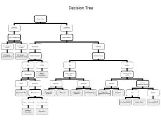
Decision Tree. LING 572 Fei Xia, Bill McNeill Week 2: 1/15/09. Main idea. Build a tree decision tree Each node represents a test Training instances are split at each node Greedy algorithm. A classification problem. Decision tree. District. Suburban (5). Urban (5). Rural (4).


Decision Tree
E N D
Presentation Transcript
Decision Tree LING 572 Fei Xia, Bill McNeill Week 2: 1/15/09
Main idea • Build a tree decision tree • Each node represents a test • Training instances are split at each node • Greedy algorithm
Decision tree District Suburban (5) Urban (5) Rural (4) House type Previous customer Respond Detached (2) Yes(3) No (2) Semi-detached (3) Nothing Nothing Respond Respond
Decision tree representation • Each internal node is a test: • Theoretically, a node can test multiple features • In most systems, a node tests exactly one feature • Each branch corresponds to test results • A branch corresponds to a feature value or a range of feature values • Each leaf node assigns • a class: decision tree • a real value: regression tree
What’s the best decision tree? • “Best”: We need a bias (e.g., prefer the “smallest” tree): • Smallest depth? • Fewest nodes? • Which trees are the best predictors of unseen data? • Occam's Razor: we prefer the simplest hypothesis that fits the data. Find a decision tree that is as small as possible and fits the data
Finding a smallest decision tree • The space of decision trees is too big for systemic search for a smallest decision tree. • Solution: greedy algorithm
Basic algorithm: top-down induction • Find the “best” feature, A, and assign A as decision feature for the node • For each value (or a range of values) of A, create a new branch, and divide up training examples • Repeat the process 1-2 until the gain is small enough
Major issues Q1: Choosing best feature: what quality measure to use? Q2: Determining when to stop splitting: avoid overfitting Q3: Handling features with continuous values
Q1: What quality measure • Any suggestions? • Information gain • Gain Ratio • 2 • Mutual information • ….
Entropy of a training set • S is a sample of training examples • Entropy is one way of measuring the impurity of S • P(ci) is the proportion of examples in S whose category is ci. H(S)=-i p(ci) log p(ci)
Information gain • InfoGain(Y | X): We must transmit Y. How many bits on average would it save us if both ends of the line knew X? • Definition: InfoGain (Y | X) = H(Y) – H(Y|X) • Also written as InfoGain (Y, X)
Information Gain • InfoGain(S, A): expected reduction in entropy due to knowing A. • Choose the A with the max information gain. (a.k.a. choose the A with the min average entropy)
S=[9+,5-] E=0.940 S=[9+,5-] E=0.940 Income PrevCustom High Low No Yes [3+,4-] [6+,2-] [6+,1-] [3+,3-] An example E=0.985 E=0.592 E=0.811 E=1.00 InfoGain (S, Income) =0.940-(7/14)*0.985-(7/14)*0.592 =0.151 InfoGain(S, PrevCustom) =0.940-(8/14)*0.811-(6/14)*1.0 =0.048
Other quality measures • Problem of information gain: • Information Gain prefers attributes with many values. • An alternative: Gain Ratio Where Sa is subset of S for which A has value a.
Q2: Avoiding overfitting • Overfitting occurs when our decision tree characterizes too much detail, or noise in our training data. • Consider error of hypothesis h over • Training data: ErrorTrain(h) • Entire distribution D of data: ErrorD(h) • A hypothesis h overfits training data if there is an alternative hypothesis h’, such that • ErrorTrain(h) < ErrorTrain(h’), and • ErrorD(h) > errorD(h’)
How to avoiding overfitting • Stop growing the tree earlier. E.g., stop when • InfoGain < threshold • Size of examples in a node < threshold • Depth of the tree > threshold • … • Grow full tree, then post-prune In practice, both are used. Some people claim that the latter works better than the former.
Post-pruning • Split data into training and validation sets • Do until further pruning is harmful: • Evaluate impact on validation set of pruning each possible node (plus those below it) • Greedily remove the ones that don’t improve the performance on validation set • Produces a smaller tree with the best performance
Performance measure • Accuracy: • on validation data • K-fold cross validation • Misclassification cost: Sometimes more accuracy is desired for some classes than others. • MDL: size(tree) + errors(tree)
Rule post-pruning • Convert the tree to an equivalent set of rules • Prune each rule independently of others • Sort final rules into a desired sequence for use • Perhaps most frequently used method (e.g., C4.5)
Q3: handling numeric features • Continuous feature discrete feature • Example • Original attribute: Temperature = 82.5 • New attribute: (temperature > 72.3) = t, f Question: how to choose split points?
Choosing split points for a continuous attribute • Sort the examples according to the values of the continuous attribute. • Identify adjacent examples that differ in their target labels and attribute values a set of candidate split points • Calculate the gain for each split point and choose the one with the highest gain.
Summary of Major issues Q1: Choosing best attribute: different quality measures. Q2: Determining when to stop splitting: stop earlier or post-pruning Q3: Handling continuous attributes: find the breakpoints
Strengths of decision tree • Simplicity (conceptual) • Efficiency at testing time • Interpretability: Ability to generate understandable rules • Ability to handle both continuous and discrete attributes.
Weaknesses of decision tree • Efficiency at training: sorting, calculating gain, etc. • Theoretical validity: greedy algorithm, no global optimization • Predication accuracy: trouble with non-rectangular regions • Stability and robustness • Sparse data problem: split data at each node.
The task • Class labels: three newsgroups (politics, mideast, and misc) • Training data: 2700 instances (900 for each class) • Test data: 300 instances (100 for each class) • Features: words • Task: • (Q1-Q3) Run Mallet DT learner • (Q4-Q5) Build your own DT learner
Q4-Q5 can take more than 10 hours. • Hw2 is a “team project”. • Each team has one or two people. • For 2-people teams: • One submission per team • Please specify the team members in your submission. • By default, the members in the same team will get the same grade.
Q4: build a DT learner • Each node checks exactly one feature • Features are all binary; that is, a feature is either present or non-present The DT is a binary tree • Quality measure: Information gain
Efficiency issue • To select the best feature, you will need to calculate the info gain for each feature • Therefore, you will need to calc the counts of (c, f) and (c, not f) for each class label c and each feature f. • Try to do this efficiently. • Report “wall clock time” in Tables 2 and 3. • When you start a job, write down the time • When the job is finished, look at the timestamp of the files • Report the difference between the two
Patas usage • When testing your code, use small data sets and small depth values first. • If your code runs more than 5 minutes, use condor submit. • Always monitor your jobs.
Addressing the weaknesses • Used in classifier ensemble algorithms: • Bagging • Boosting • Decision tree stump: one-level DT
Other issues Q4: Handling training data with missing feature values Q5: Handing features with different costs • Ex: features are medical test results Q6: Dealing with y being a continuous value
Q4: Unknown attribute values Possible solutions: • Assume an attribute can take the value “blank”. • Assign most common value of A among training data at node n. • Assign most common value of A among training data at node n which have the same target class. • Assign prob pi to each possible value vi of A • Assign a fraction (pi) of example to each descendant in tree • This method is used in C4.5.
Q5: Attributes with cost • Ex: Medical diagnosis (e.g., blood test) has a cost • Question: how to learn a consistent tree with low expected cost? • One approach: replace gain by • Tan and Schlimmer (1990)
Q6: Dealing with continuous target attribute Regression tree • A variant of decision trees • Estimation problem: approximate real-valued functions: e.g., the crime rate • A leaf node is marked with a real value or a linear function: e.g., the mean of the target values of the examples at the node. • Measure of impurity: e.g., variance, standard deviation, …
Summary of other issues Q4: Handling training data with missing attribute values: blank value, most common value, or fractional count Q5: Handing attributes with different costs: use a quality measure that includes the cost factors. Q6: Dealing with continuous goal attribute: various ways of building regression trees.
Summary • Basic case: • Discrete input attributes • Discrete target attribute • No missing attribute values • Same cost for all tests and all kinds of misclassification. • Extended cases: • Continuous attributes • Real-valued target attribute • Some examples miss some attribute values • Some tests are more expensive than others.
Common algorithms • ID3 • C4.5 • CART
ID3 • Proposed by Quinlan (so is C4.5) • Can handle basic cases: discrete attributes, no missing information, etc. • Information gain as quality measure
C4.5 • An extension of ID3: • Several quality measures • Incomplete information (missing attribute values) • Numerical (continuous) attributes • Pruning of decision trees • Rule derivation • Random mood and batch mood
CART • CART (classification and regression tree) • Proposed by Breiman et. al. (1984) • Constant numerical values in leaves • Variance as measure of impurity